
QC Scope is a plugin for FIJI designed to process microscope images for Quality Control purposes.
Written by Nicolas Stifani from the Centre d'Innovation Biomédicale de la Faculté de Médecine de l'Université de Montréal.
Field Uniformity
Usage
- Open FIJI.
- Launch the QC Scope Toolbar by navigating to Plugins>QC Scope>QC Scope Toolbar.
- Click on Uniformity.
- If one or more images are already opened QC Scope will process them.
- If no image is open, QC Scope will prompt to select a folder and process all images withing the folder (and subfolders)
- QC Scope will try to read the Metadata from the first image and pre-process all the channels with default or the last used processing settings
- It will display the metadata, the initial results and the processing options in a dialog
- Check the metadata, the results and the binned image. If it looks good you can click OK.
QC Scope will save files in a folder named Output on your desktop:
At least 2 CSV files:
- Field Uniformity_All-Data_Merged.csv gathers all the measured parameters
Field Uniformity_All-Data_Merged.csv Field Uniformity_Essential-Data_Merged.csv gathers only the essential information
Field Uniformity_Essential-Data_Merged.csv
- Field Uniformity_All-Data_Merged.csv gathers all the measured parameters
- Optionally, if Save Individual Files is selected QC Scope will also save:
- 1 CSV file per image ImageName_Uniformity-Data.csv with one row per channel containing all the measured parameters
- 1 TIF file per channel for every processed image showing the binned (Iso-density or Iso-Intensity) map with the Reference Center indicated as an overlay

Example of iso-density image with the coordinates of the reference center.
Settings
- Microscope Settings read from the image metadata or from the preferences: Objective Magnification (character), NA (Numeric>0), and Immersion media
- Image Settings: Pixel Width (Numeric>0), Height (Numeric>0), Depth (Voxel) (Numeric>0), Unit (character). QC Scope uses standard space unit (nm, um, mm, cm, m, in, pixels) and will try to convert the entered value into on of those.
- Channel Settings: For each channel: Name (character) and Emission Wavelength in nm ((Numeric>0)) as well as the source of the values
- Processing Settings:
- Binning Method:
- Iso-Density (preferred): This method divides the image into 10 bins of equal Nb of Pixels. Nb Pixel Per Bin = (Width x Height) / 10 and assign a new pixel value of 25 for all the Nb Pixel Per Bin darkest pixels, 50 for the next darkest Nb Pixel Per Bin etc... until 250 for the brightest Nb Pixel Per Bin pixels.
- Iso-Intensity: This method divides the image into 10 bins of equal bin intensities. Bin Width = (Max - Min) / 10 and assign a new pixel value of 25 for all the pixels with an intensity between Min and Min + Bin With, 50 for intensities between Min + Bin Width and Min + 2 x Bin Width etc... until 250 for intensities between Min + 9 x Bin Width and Max.
- Gaussian Blur: Apply a Gaussian blur with the given Gaussian Blur Sigma before processing each channel
- Channel: The selected channel will be processed with the entered processing parameters and displayed as part of the testing process to define optimal processing parameters.
- Batch Mode: If activated, QC Scope will re-use the settings without displaying the dialog unless metadata differs
- Save Individual Files: For each image, QC Scope will save the individual processed images (1 per channel) and a CSV file with all measured parameters.
- Prolix Mode: Display all the QC Scope actions in the log
Test Processing: When selected the QC Scope Field Uniformity Dialog will keep appearing. This is useful to test the Processing Settings. When you are satisfied you can uncheck Test processing to proceed to the next image.
- Binning Method:

QC Scope Field Uniformity dialog
Results
- Convert the Field Uniformity_Essential-Data_Merged.csv created by QC Scope Field Uniformity function into a .xlsx
- Summarize the data with a pivot table
- Use the provided spreadsheet template Field Uniformity_Template.xlsx
- Enter your measurement into the highlighted cells of the template to visualize your results. The cells in grey are automatically computed.
- Plot the Field illumination Index for each objective and filter combination
The 2x, 20x and 63x objectives have a field illumination index above 70% for all filters indicating an acceptable uniformity and centering accuracy. The 10x objective field illumination index is below 70% indicating a poor uniformity and/or Centering accuracy requiring further investigations.
- Plot the Uniformity and Centering Accuracy for each objective and filter combination


All objectives show a good Uniformity. The 2x, 10x and 20x objectives have a centering accuracy below 70% indicating a poor illumination centering.


Iso-density map showing the localization of the centroid of the highest intensity bin for 10x and 63x objectives.

Field illumination Index for each objective and filter combination
Channel Alignment
Usage
- Open FIJI.
- Launch the QC Scope Toolbar by navigating to Plugins>QC Scope>QC Scope Toolbar.
- Click on Ch Alignment.
- If one or more images are already opened QC Scope will process them.
- If no image is open, QC Scope will prompt to select a folder and process all images withing the folder (and subfolders)
- QC Scope will try to read the Metadata from the first image and pre-process all the channels with the default or the last used processing settings
- It will display the metadata, the initial results and the processing options in a dialog
- Check the metadata and the results. If it looks good you can click OK. You can also modify the the metadata and processing options
QC Scope will save files in a folder named Output on your desktop:
At least 2 CSV files are saved :
- Channel-Alignment_All-Data_Merged.csv gathers all the measured parameters
Channel Alignment_All-Data_Merged.csv Channel Alignment_Essential-Data_Merged.csv gathers only the essential information
Channel Alignment_Essential-Data_Merged.csv
- Channel-Alignment_All-Data_Merged.csv gathers all the measured parameters
- Optionally, if Save Individual Files is selected QC Scope will also save:
- 1 CSV file per image gathering all the measured parameters for each channel pair (Image-Name_Channel-Alignment_All-Data.csv)

Settings
- Microscope Settings: Read from the image metadata or from the preferences: Objective Magnification (character), NA (Numeric>0), and Immersion media
- Image Settings: Read from the image Calibration. Pixel Width (Numeric>0), Height (Numeric>0), Depth (Voxel) (Numeric>0), Unit (character). QC Scope uses standard space unit (nm, um, mm, cm, m, in, pixels) and will try to convert the entered value into one of those.
- Channel Settings: Read from the image metadata or from the preferences, for each channel: Name (character) and Emission Wavelength in nm ((Numeric>0)) as well as displaying the source of the values
- Processing Settings:
- Detection Method:
- Log Detector: Laplacian of Gaussian (LoG) detector. From Trackmate: The LoG detector is the best detector for Gaussian-like particles in the presence of noise. It is based on applying a LoG filter on the image and looking for local maxima. The Laplacian of Gaussian result is obtained by summing the second order spatial derivatives of the gaussian- filtered image, and normalizing for scale. Reference: Trackmate manual (page 52).
- Dog Detector: Difference of Gaussian (DoG) detector. From Trackmate: This detector is based on the Difference of Gaussian (DoG) filter. It approximates the Laplacian of Gaussian (LoG) filter with the aim at offering better speed. It is commonly used when applying a collection of DoG filters tuned to a wide range of scales. Reference: Trackmate manual (page 52).
- Threshold: This is a quality threshold. Only spots above the quality threshold will be detected. The quality value is larger for : Bright spots, spots which diameter is close to the specified diameter.
- Diameter: This is the diameter for the detection of spots with the indicated unit. Usually this is the diameter of the beads used for the channel alignment.
- Median Filtering: If activated QC Scope will ask Trackmate to use a Median Filtering. Median filtering: will apply a 3 x 3 median filter prior to any processing.
This can help dealing with images that have a marked salt and pepper noise which generates spurious spots. Reference: Trackmate manual (page 11). - Channel: The selected channel will be processed with the entered processing parameters and displayed as part of the testing process to define optimal processing parameters. Selecting an another channel will automatically enable Test Processing.
- Batch Mode: If activated, QC Scope will re-use the settings without displaying the dialog unless metadata differs or the detection fails.
- Save Individual Files: If activated, QC Scope will save an additional CSV File per image named Image-Name_Channel-Alignment_All-Data.csv gathering all the measured parameters for each channel pair (1 row per channel pair = Nb Channel2 rows per file.
- Prolix Mode: Display all the QC Scope actions in the log. If used in combination with Save Individual Files, it will save the original Trackmate spot table (1 per channel)
- Subpixel Precision: If activated QC Scope will ask Trackmate to use a subpixel localization for the detection of spots
Test Processing: When selected the QC Scope Dialog will keep appearing. This is useful to test the Processing Settings. When you are satisfied you can uncheck Test processing to proceed to the next image. Changing the selected channel automatically select the Test Processing option.
- Detection Method:
- Pre-detection results:
- Nb of Detected spots: Indicate the number of detected spot per channel. To proceed, exactly one spot must be detected for every channel.
- Max Quality: Indicate the maximum quality of all detected spots for each channel. The maximum quality can then be used to adjust the threshold value
Results
- Convert the Channel Alignment_Essential-Data_Merged.csv created by QC Scope Channel Alignment function into a .xlsx
- Summarize the data with a pivot table
- Use the provided spreadsheet template Channel Alignment_Template.xlsx
- Paste the Colocalization Ratio and the XYZ pixel shifts in the Shift Tab. The cells use conditional formatting to highlight cells with a ratio above 1.0.


These results indicates that the 63x objective requires correction for the DAPI channel. User should be informed to correct the images.
 63x DAPI (Cyan) and Cy5 (Magenta) 4um bead raw image.
 63x DAPI (Cyan) and Cy5 (Magenta) 4um bead corrected for chromatic shift.

63x DAPI (Cyan) and Cy5 (Magenta) 4um bead Z-Stack.

63x DAPI (Cyan) and Cy5 (Magenta) 4um bead Z-Stack corrected for chromatic shift.

This page provides a practical guide for microscope quality control. By following the outlined steps, utilizing the provided template files, and running the included scripts, you will have everything needed to easily generate comprehensive report on your microscope's performance.
Equipment used
- Thorlabs Power Meter (PM400) and sensor (S170C)
- Thorlabs Fluorescent Slides (FSK5)
- TetraSpeck™ Fluorescent Microspheres Size Kit (mounted on slide) ThermoFisher (T14792)
Software used
- FIJI FIJI
QC Scope Plugin for FIJI
- MetroloJ_QC Plugin for FIJI
- iText Plugin for FIJI (required for MetroloJ_QC)
- R from the CRAN R Project
- I typically use RStudio the integrated development environment (IDE) for R
- Bulk Rename Utility s a powerfull mini software to rename your files.
Excel Templates and Scripts
Please note that during quality control, you may, and likely will, encounter defects or unexpected behavior. This practical guide is not intended to assist with investigating or resolving these issues. With that said, we wish you the best of luck and are committed to providing support. Feel free to reach out to us at microscopie@cib.umontreal.ca
Illumination Warmup Kinetic
When starting light sources, they require time to reach a stable and steady state. This duration is referred to as the warm-up period. To ensure accurate performance, it is essential to record the warm-up kinetics at least once a year to precisely define this period. For a detailed exploration of illumination stability, refer to the Illumination Power, Stability, and Linearity Protocol by the QuaRep Working Group 01.
Acquisition protocol
Results
- Use the provided spreadsheet template, Illumination_Warmup Kinetic_Template.xlsx
- Copy and paste the data from the recorded CSV file into the highlighted cells of the template to visualize your results.
- For each light source, plot the measured power output (in mW) against time to analyze the data.

- Calculate the relative power using the formula: Relative Power = (Power / Max Power) for each wavelength. Then, plot the Relative Power (%) against Time to visualize the data.

We observe some variability in the power output during the first 20 min. It is especially noticeable for the 385 nm light source.
To assess the stability:
Define a Stability Duration Window: This is a time period (e.g., 10 minutes) during which the power output should remain stable.
Specify a Maximum Coefficient of Variation (CV) Threshold: This a limit acceptable for the CV (e.g., 0.01%).
Calculate the Coefficient of Variation (CV): CV = (Standard Deviation / Mean)
Plot the calculated CV over time to analyze the stability of the power output.


We observe that most of light sources stabilize quickly, within less than 10 minutes, while the 385 nm light source takes approximately 41 minutes to reach the stability threshold. The template also calculates Stability Factor (S) using the formula: S (%) = 100 × (1 - (Pmax - Pmin) / (Pmax + Pmin))
- Report the results in a table
| 385nm | 475nm | 555nm | 630nm | |
Stabilisation time (Max CV 0.01% for 10 min) | 41 | 3 | 3 | 8 |
| Stability Factor (%) Before Warmup | 99.7% | 99.9% | 100.0% | 100.0% |
| Stability Factor (%) After Warmup | 100.0% | 100.0% | 100.0% | 99.9% |
Metrics
- The Stability Factor indicates a higher stability the closer to 100% and focuses specifically on the range of values (difference between max and min) relative to their sum, providing an intuitive measure of how tightly the system's behavior stays within a defined range.
- The Coefficient of Variation focuses on the dispersion of all data points (via the standard deviation) relative to the mean. Lower Coefficient indicates a better stability around the mean.
Conclusion
Illumination Maximum Power Output
This measure assesses the maximum power output of each light source, considering both the quality of the light source and the components along the light path. Over time, we expect a gradual decrease in power output due to the aging of hardware, including the light source and other optical components. These measurements will also be used to track the performance of the light sources over their lifetime (see Long-Term Illumination Stability section). For a detailed exploration of illumination properties, refer to the Illumination Power, Stability, and Linearity Protocol by the QuaRep Working Group 01.
Acquisition protocol
Results
- Use the provided spreadsheet template Illumination_Maximum Power Output_Template.xlsx
- Fill in the highlighted cells of the template to visualize your results.
- For each light source, plot the measured Maximum Power Output (in mW).

These results are informative on their own but could become even more meaningfull when comapred to the manufacturer’s specifications.
- Calculate the Relative PowerSpec using the formula: Relative PowerSpec = (Measured Power / Manufacturer Specifications) and plot the Relative Power for each light source.

- Report the results in a table
| Manufacturer Specifications (mW) | Measurements 2024-11-22 (mW) | Relative PowerSpec (%) | |
| 385nm | 150.25 | 122.2 | 81% |
| 470nm | 110.4 | 95.9 | 87% |
| 555nm | 31.9 | 24 | 75% |
| 630nm | 52 | 39.26 | 76% |
Metrics
- The Maximum Power indicates how much light is provided by the instrument.
- The Relative PowerSpec indicates how much power is provided compared to the specifications.
Conclusion
Illumination Stability
The light sources used on a microscope should remain constant or at least stable over the time scale of an experiment. For this reason, illumination stability is recorded across four different time scales:
- Real-time Illumination Stability: Continuous recording for 1 minute. This represents the duration of a z-stack acquisition.
- Short-term Illumination Stability: Recording every 1-10 seconds for 5-15 minutes. This represents the duration needed to acquire several images.
- Mid-term Illumination Stability: Recording every 10-30 seconds for 1-2 hours. This represents the duration of a typical acquisition session or short time-lapse experiments. For longer time-lapse experiments, a longer duration may be used.
- Long-term Illumination Stability: Recording once a year or more over the lifetime of the instrument.
For a detailed exploration of illumination stability, refer to the Illumination Power, Stability, and Linearity Protocol by the QuaRep Working Group 01.
Real-time Illumination Stability
Acquisition protocol
Results
- Use the provided spreadsheet template Illumination_Stability_Template.xlsx
- Copy and paste the data from the recorded CSV file into the highlighted cells of the template to visualize your results.
- For each light source, plot the Measured Power Output (in mW) over Time.

- Calculate the Relative Power using the formula: Relative Power = (Power / Max Power). Then, plot the Relative Power (%) over Time.

- Calculate the Stability Factor (S) using the formula: S (%) = 100 × (1 - (Pmax - Pmin) / (Pmax + Pmin)).
- Calculate the Coefficient of Variation (CV) using the formula: CV = Standard Deviation / Mean.
- Reports the results in a table.
| Stability Factor | Coefficient of Variation | |
| 385nm | 99.99% | 0.002% |
| 475nm | 99.99% | 0.002% |
| 555nm | 99.97% | 0.004% |
| 630nm | 99.99% | 0.002% |
From the Stability Factor results, we observe that the difference between the maximum and minimum power is less than 0.03%. Additionally, the Coefficient of Variation indicates that the standard deviation is less than 0.004% of the mean value, demonstrating excellent realtime power stability.
Conclusion
Short-term Illumination Stability
Acquisition protocol
Results
- Use the provided spreadsheet template Illumination_Stability_Template.xlsx
- Copy and paste the data from the recorded CSV file into the highlighted cells of the template to visualize your results.
- For each light source, plot the Measured Power Output (in mW) over Time.

- Calculate the Relative Power using the formula: Relative Power = (Power / Max Power). Then, plot the Relative Power (%) over Time.

- Calculate the Stability Factor (S) using the formula: S (%) = 100 × (1 - (Pmax - Pmin) / (Pmax + Pmin)).
- Calculate the Coefficient of Variation (CV) using the formula: CV = Standard Deviation / Mean.
- Reports the results in a table.
| Stability Factor | Coefficient of Variation | |
| 385nm | 100.00% | 0.000% |
| 475nm | 100.00% | 0.002% |
| 555nm | 100.00% | 0.003% |
| 630nm | 99.99% | 0.004% |
From the Stability Factor, we observe that the difference between the maximum and minimum power is less than 0.01%. Additionally, the Coefficient of Variation indicates that the standard deviation is less than 0.004% of the mean value, demonstrating excellent short-term power stability.
Conclusion
Mid-term Illumination Stability
Acquisition protocol
Results
- Use the provided spreadsheet template Illumination_Stability_Template.xlsx
- Copy and paste the data from the recorded CSV file into the highlighted cells of the template to visualize your results.
- For each light source, plot the Measured Power Output (in mW) over Time

- Calculate the Relative Power using the formula: Relative Power = (Power / Max Power). Then, plot the Relative Power (%) over Time.

- Calculate the Stability Factor (S) using the formula: S (%) = 100 × (1 - (Pmax - Pmin) / (Pmax + Pmin)).
- Calculate the Coefficient of Variation (CV) using the formula: CV = Standard Deviation / Mean.
- Reports the results in a table.
| Stability Factor | Coefficient of Variation | |
| 385nm | 99.98% | 0.013% |
| 475nm | 99.98% | 0.011% |
| 555nm | 99.99% | 0.007% |
| 630nm | 99.97% | 0.020% |
From the Stability Factor, we observe that the difference between the maximum and minimum power is less than 0.03%. Additionally, the Coefficient of Variation indicates that the standard deviation is less than 0.02% of the mean value, demonstrating excellent mid-term power stability.
Conclusion
Long-term Illumination Stability
Long-term illumination stability measures the power output over the lifetime of the instrument. Over time, we expect a gradual decrease in power output due to the aging of hardware, including the light source and other optical components. These measurements are not an experiment per se but it is the measurement of the maximum power output over time.
Acquisition protocol
Results
- Use the provided spreadsheet template Illumination_Long-Term_Stability_Log.xlsx
- Copy and paste the data from the recorded CSV file into the highlighted cells of the template to visualize your results.
- For each light source, plot the Measured Power Output (in mW) over Time
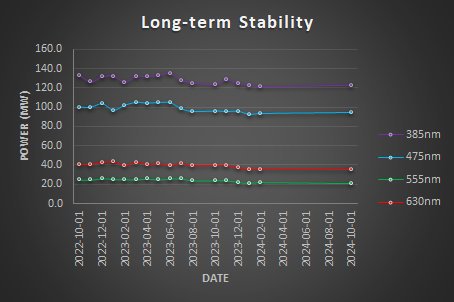
- Calculate the Relative Power using the formula: Relative Power = (Power / Max Power). Then, plot the Relative Power (%) over Time.

- Calculate the Relative PowerSpec by comparing the measured power to the manufacturer’s specifications using the following formula: Relative PowerSpec = Power / PowerSpec
- Plot the Relative PowerSpec (% Spec) over Time.

We expect a gradual decrease in power output over time due to the aging of hardware. Light sources should be replaced when the Relative PowerSpec falls below 50%.
- Reports the results in a table.
| Relative PowerSpec | |
| 385nm | 80.53% |
| 475nm | 83.61% |
| 555nm | 65.83% |
| 630nm | 67.12% |
- Keep the Log file to append future measurements
Conclusion
Illumination Stability Conclusions
| Stability Factor | Real-time 1 min | Short-term 15 min | Mid-term 1 h |
385nm | 99.99% | 100.00% | 99.98% |
475nm | 99.99% | 100.00% | 99.98% |
555nm | 99.97% | 100.00% | 99.99% |
630nm | 99.99% | 99.99% | 99.97% |
The light sources are highly stable (Stability >99.9%).
Metrics
- The Stability Factor indicates a higher stability the closer to 100% and focuses specifically on the range of values (difference between max and min) relative to their sum, providing an intuitive measure of how tightly the system's behavior stays within a defined range.
- The Coefficient of Variation focuses on the dispersion of all data points (via the standard deviation) relative to the mean. Lower Coefficient indicates a better stability around the mean.
Illumination Input-Output Linearity
This measure compares the power output as the input varies. A linear relationship is expected between the input and the power output. For a detailed exploration of illumination linearity, refer to the Illumination Power, Stability, and Linearity Protocol by the QuaRep Working Group 01.
Acquisition protocol
Results
- Use the provided spreadsheet template Illumination_Linearity_Template.xlsx
- Enter your measurement into the highlighted cells of the template to visualize your results.
- For each light source, plot the Measured Power output (in mW) as a function of the Input (%).

- Calculate the Relative Power using the formula: Relative Power = Power / MaxPower.
- Plot the Relative Power (%) as a function of the Input (%).

- Determine the equation for each curve, which is typically a linear relationship of the form: Output = K × Input
- Report the Slope (K) and the Coefficient of Determination (R²) for each curve in a table.
Illumination Input-Output Linearity | ||
Slope | R2 | |
385nm | 0.9969 | 1 |
475nm | 0.9984 | 1 |
555nm | 1.0012 | 1 |
630nm | 1.0034 | 1 |
The slopes demonstrate a nearly perfect linear relationship between the input and the measured output power, with values very close to 1. The coefficient of determination (R²) indicates a perfect linear fit, showing no deviation from the expected relationship.
Metrics
- The Slope indicates the rate of change between Input and Ouput.
- The Coefficient of Determination indicates how fitted is the data to a linear relationship.
Conclusion
Objectives and Cubes Transmittance
Since we are using a power meter, we can easily assess the transmittance of the objectives and filter cubes. This measurement compares the power output when different objectives and filter cubes are in the light path. It evaluates the transmittance of each objective and compares it with the manufacturer’s specifications. This method can help detect defects or dirt on the objectives. It can also verify the correct identification of the filters installed in the microscope.
Objectives Transmittance
Acquisition protocol
Results
- Use the provided spreadsheet template Objective and cube transmittance_Template.xlsx
- Enter your measurement into the highlighted cells of the template to visualize your results.
- For each light source, plot the Measured Power output (in mW) as a function of the wavelength (in nm).

- Calculate the Relative Transmittance using the formula: Relative Transmittance = Power / PowerNoObjective.
- Plot the Relative Transmittance (%) as a function of the wavelength (in nm).

- Calculate the average transmittance for each objective
- Compare the average transmittance to the specifications provided by the manufacturer
- Report results in a table.
| Average Transmittance | Specifications [470-630] | Average Transmittance | |
| 2.5x-0.075 | 77% | >90% | 84% |
| 10x-0.25-Ph1 | 60% | >80% | 67% |
| 20x-0.5 Ph2 | 62% | >80% | 68% |
| 63x-1.4 | 29% | >80% | 35% |
The measurements are generally close to the specifications, with the exception of the 63x-1.4 objective. This deviation is expected, as the 63x objective has a smaller back aperture, which reduces the amount of light it can receive..
Conclusion
Cubes Transmittance
Acquisition protocol
Results
- Use the provided spreadsheet template Objective and cube transmittance_Template.xlsx
- Enter your measurement into the highlighted cells of the template to visualize your results.
- For each light source, plot the Measured Power output (in mW) as a function of the wavelength (in nm)..

- Calculate the Relative Transmittance using the formula: Relative Transmittance = Power / PowerMaxFilter.
- Plot the Relative Transmittance (%) as a function of the wavelength (in nm).

- Calculate the Average Transmittance for each filter at the appropriate wavelengths
- Report the results in a table.
| 385 | 475 | 555 | 590 | 630 | |
| DAPI/GFP/Cy3/Cy5 | 100% | 100% | 100% | 100% | 100% |
| DAPI | 14% | 0% | 0% | 8% | 0% |
| GFP | 0% | 47% | 0% | 0% | 0% |
| DsRed | 0% | 0% | 47% | 0% | 0% |
| DHE | 0% | 0% | 0% | 0% | 0% |
| Cy5 | 0% | 0% | 0% | 0% | 84% |
The DAPI cube transmits only 14% of the excitation light compared to the Quad Band Pass DAPI/GFP/Cy3/Cy5. While it is still usable, it will provide a low signal. This is likely because the excitation filter within the cube does not match the light source properly. Since an excitation filter is already included in the light source, the filter in this cube could be removed.
The GFP and DsRed cubes transmit 47% of the excitation light compared to the Quad Band Pass DAPI/GFP/Cy3/Cy5, and they are functioning properly.
The DHE cube does not transmit any light from the Colibri. This cube may need to be removed and stored.
The Cy5 cube transmits 84% of the excitation light compared to the Quad Band Pass DAPI/GFP/Cy3/Cy5, and it is working properly.
Conclusion
We are done with the powermeter ![]() .
.
Field Illumination Uniformity
Having confirmed the stability of our light sources and verified that the optical components (objectives and filter cubes) are transmitting light effectively, we can now proceed to evaluate the uniformity of the illumination. This step assesses how evenly the illumination is distributed. For a comprehensive guide on illumination uniformity, refer to the Illumination Uniformity by the QuaRep Working Group 03.
Acquisition protocol
Processing
You should have acquired several multi-channel images that now need processing to yield meaningful results.
I initially was using the Field Illumination analysis function of the MetroloJ_QC plugin for FIJI but eventually branched away to write my own processing plugin named QC Scope. For more information about the QC Scope please refer to the QC Scope repository on Github. For more information about MetroloJ_QC plugin please refer to manual available on the MontpellierRessourcesImagerie repository on GitHub.
- Open FIJI.
- Launch the QC Scope Toolbar by navigating to Plugins>QC Scope>QC Scope Toolbar.
- Click on Uniformity.
- If one or more images are already opened QC Scope will process them.
- If no image is open, QC Scope will prompt to select a folder and process all images withing the folder (and subfolders)
QCSCope file format compatibility
For now, QC Scope only processes images with the following extensions ".tif", ".tiff", ".jpg", ".jpeg", ".png", ".czi", ".nd2", ".lif", ".lsm", ".ome.tif", ".ome.tiff"
- QC Scope will try to read the Metadata from the first image and pre-process all the channels with default or the last used processing settings
- It will display the metadata, the initial results and the processing options in a dialog
- Microscope Metadata: Objective Magnification, NA, and Immersion media
- Image Calibration status, Pixel Width, Height, Voxel Size, Unit
- For each channel: Name and Emission Wavelength
- Processing Settings:
- Binning Method:
- Iso-Density (preferred): This method divides the image into 10 bins of equal Nb of Pixels. Nb Pixel Per Bin = (Width x Height) / 10 and assign a new pixel value of 25 for all the Nb Pixel Per Bin darkest pixels, 50 for the next darkest Nb Pixel Per Bin etc... until 250 for the brightest Nb Pixel Per Bin pixels.
- Iso-Intensity: This method divides the image into 10 bins of equal bin intensities. Bin Width = (Max - Min) / 10 and assign a new pixel value of 25 for all the pixels with an intensity between Min and Min + Bin With, 50 for intensities between Min + Bin Width and Min + 2 x Bin Width etc... until 250 for intensities between Min + 9 x Bin Width and Max.
- Gaussian Blur: Apply a gaussian blur with the given Gaussian Blur Sigma before processing the image channel
- Channel: The selected channel will be processed with the entered processing parameters and displayed as part of the testing process to define optimal processing parameters.
- Batch Mode: If activated, QC Scope will re-use the settings without displaying the dialog unless metadata differs
- Save Individual Files: For each image, QC Scope will save the individual processed images (1 per channel) and a CSV file with all measured parameters.
- Prolix Mode: Display all the QC Scope actions in the Log
Test Processing: When selected the Dialog will keep appearing. This is useful to test the Processing Settings

- Binning Method:
QC Scope will save files in a folder named Output on your desktop:
At least 2 CSV files:
- Field Uniformity_All-Data_Merged.csv gathers all the measured parameters
Field Uniformity_Essential-Data_Merged.csv gathers only the essential information
- Optionnally, if Save Individual Files is selected QC Scope will also save:
- 1 CSV file per image NameOfYourImage_Uniformity-Data.csv with one row per channel containing all the measured parameters
- 1 TIF file per channel for every processed image showing the binned (Iso-density or Iso-Intensity) image map with the Reference Center indicated as an overlay
Note: QC Scope never overwrites files. It will check for the existence of files and increment a number until it can safely write the output file.
Description of QC Scope Field Uniformity Results (in bold the results included in Essential Data)
| Key Order | Field Name | Data Example | Data Type | Description |
| 1 | Filename | 10x_Quad_Exp-01.czi | String | Name of the processed image |
| 2 | Channel Nb | 4 | Integer | Number of the Channel from 1 to n |
| 3 | Channel Name | DAPI | String | Name of the Channel |
| 4 | Channel Wavelength EM (nm) | 465 | Integer | Channel Emission Wavelength |
| 5 | Objective Magnification | 10x | String | Objective Magnification |
| 6 | Objective NA | 0.25 | Float | Objective Numerical Aperture |
| 7 | Objective Immersion Media | Air | String | Objective Immerion Media |
| 8 | Gaussian Blur Applied | TRUE | Boolean | If Gaussian Blur was applied |
| 9 | Gaussian Sigma | 10 | Integer | Sigma of the Gaussian Blur |
| 10 | Binning Method | Iso-Density | String | Binning Method used |
| 11 | Batch Mode | TRUE | Boolean | Boolean key to process images in batch mode (no Dialog) |
| 12 | Save Individual Files | FALSE | Boolean | Boolean key to save individual files (1 csv data per file with 1 row per channel, 1 tif binned image par channel) |
| 13 | Prolix Mode | FALSE | Boolean | Boolean key display detailed plugin actions in the log |
| 14 | Image Min Intensity | 856 | Integer | Raw Image Minimum of Pixel Intensities |
| 15 | Image Max Intensity | 1080 | Integer | Raw Image Maximum of Pixel Intensities |
| 16 | Image Mean Intensity | 959.1 | Float | Raw Image Mean of Pixel Intensities |
| 17 | Image Standard Deviation Intensity | 24.3 | Float | Raw Image Standard Deviation of Pixel Intensities |
| 18 | Image Median Intensity | 959 | Integer | Raw Image Median Pixel Intensity |
| 19 | Image Mode Intensity | 110 | Integer | Raw Image Mode Pixel Intensity |
| 20 | Image Width (pixels) | 1388 | Integer | Image Width in pixels |
| 21 | Image Height (pixels) | 1040 | Integer | Image Height in pixels |
| 22 | Image Bit Depth | 16 | Integer | Image Bit Depth |
| 23 | Pixel Width (um) | 0.645 | Float | Image pixel width (unit/px) |
| 24 | Pixel Height (um) | 0.645 | Float | Image pixel height (unit/px) |
| 25 | Pixel Depth (um) | 1 | Float | Image voxel depth (unit/voxel) |
| 26 | Space Unit | micron | String | Raw Image Space Unit |
| 27 | Space Unit Standard | um | String | Standardize Space Unit (nm, um, cm, m) |
| 28 | Calibration Status | TRUE | Boolean | Boolean key displaying the calibration status |
| 29 | Standard Deviation (GV) | 24.3 | Float | Raw Image Standard Deviation of Pixel Intensities |
| 30 | Uniformity Standard (%) | 79.3 | Float | Uniformity as calculated by MetroloJ_QC. Uniformity_Standard = 100 * (Min / Max) |
| 31 | Uniformity Percentile (%) | 95.8 | Float | Uniformity calculated with the average of the 5% and 95% pixel intensities. Uniformity_Percentile = (1 - (Avg_Intensity95 - Avg_Intensity5) / (Avg_Intensity95 + Avg_Intensity5) ) * 100 |
| 32 | Coefficient of Variation | 0.0253 | Float | Coefficient of variation. CV = (Std_Dev / Mean) |
| 33 | Uniformity CV based | 97.5 | Float | Uniformity calculated from the Coefficient of variation. Uniformity_CV = (1 - CV) * 100 |
| 34 | X Center (pixels) | 694 | Integer | Coordinate in pixel of the center of the Image (Ideal centering). Image Width (pixels) / 2 |
| 35 | Y Center (pixels) | 520 | Integer | Coordinate in pixel of the center of the Image (Ideal centering). Image Height (pixels) / 2 |
| 36 | X Ref (pixels) | 230.4 | Float | Coordinate in pixels of the centroid of the largest particule identified in the last bin. Used to caculate the Centering Accuracy |
| 37 | Y Ref (pixels) | 876.4 | Float | Coordinate in pixels of the centroid of the largest particule identified in the last bin. Used to caculate the Centering Accuracy |
| 38 | X Ref (um) | 148.6 | Float | Coordinate in scaled unit of the centroid of the largest particule identified in the last bin. |
| 39 | Y Ref (um) | 565.3 | Float | Coordinate in scaled unit of the centroid of the largest particule identified in the last bin. |
| 40 | Centering Accuracy (%) | 32.6 | Float | Centering Accuracy = 100 - 100 * (2 / sqrt(Image Width**2 + Image Height**2)) * sqrt ( (X_Ref_Pix - Image Width/2)**2 + (Y_Ref_Pix - Image Height/2)**2) |
Results
Plot the uniformity and centering accuracy for each objective.
Metrics
- The Uniformity indicates the range between the minimum and maximum intensities in the image. U=(Min/Max)*100. 100% Uniformity indicates a perfectly homogeneous image. 50% Uniformity indicates the minimum is half the maximum.
- The Centering Accuracy indicates how far from the center of the image is the center of the illumination (centroid of the max illumination bin). 100% indicates a perfectly aligns with the center of the image. 0% centering accuracy indicates that the center of the illumination is the farthest from the center of the image.

| Objective | Uniformity | Centering Accuracy |
| 2x | 97.5% | 92.7% |
| 10x | 97.0% | 94.5% |
| 20x | 97.3% | 97.1% |
| 63x | 96.6% | 96.7% |
Plot the uniformity and centering accuracy for each filter set.

| Filter | Uniformity | Centering Accuracy |
| DAPI | 98.3% | 99.4% |
| DAPIc | 95.8% | 84.9% |
| GFP | 98.1% | 99.1% |
| GFPc | 96.5% | 93.3% |
| Cy3 | 97.6% | 96.5% |
| Cy3c | 96.8% | 97.9% |
| Cy5 | 97.0% | 99.6% |
| Cy5c | 96.7% | 91.3% |
This specific instrument has a quad-band filter as well as individual filter cubes. We can plot the uniformity and centering accuracy per filter types.

| Filter Type | Uniformity | Centering Accuracy |
Quad band | 97.7% | 98.7% |
| Single band | 96.5% | 91.8% |
Conclusion
XYZ Drift
This experiment evaluates the stability of the system in the XY and Z directions. As noted earlier, when an instrument is started, it requires a warmup period to reach a stable steady state. To determine the duration of this phase accurately, it is recommended to record a warmup kinetic at least once per year. For a comprehensive guide on Drift and Repositioning, refer to the Stage and Focus Precision by the QuaRep Working Group 06.
Acquisition protocol
Processing
Results
- Open the spreadsheet template XYZ Drift Kinetic_Template.xlsx and fill in the orange cells.
- Copy and paste the XYZT and Frame columns from the TrackMate spots CSV file into the corresponding orange columns in the spreadsheet.
- Enter the numerical aperture (NA) and emission wavelength used during the experiment.
- Calculate the relative displacement in X, Y, and Z using the formula: Relative Displacement = Position - PositionInitial.
- Finally, plot the relative displacement over time to visualize the system's drift.


Identify visually the time when the displacement is lower than the resolution of the system. On this instrument it takes 120 min to reach its stability. Calculate the velocity, Velocity = (Displacement2-Displacement1)/T2-T1) and plot the velocity over time.

Calculate the average velocity before and after stabilisation and report the results in a table.
| Objective NA | 0.5 |
| Wavelength (nm) | 705 |
| Resolution (nm) | 705 |
| Stabilisation time (min) | 122 |
| Average velocity Warmup (nm/min) | 113 |
| Average velocity System Ready (nm/min) | 14 |
Metrics
- The Stabilisation Time indicates the time in minutes necessary for the instrument to have a drift lower than the resolution of the system.
- The Average Velocity indicates the speed of drift in all directions XYZ in nm/min.
Conclusion
Stage Repositioning Dispersion
This experiment evaluates how accurate is the system in XY by measuring the dispersionof repositioning. Several variables can affect repositioning: i) Time, ii) Traveled distance, iii) Speed and iv) acceleration. For a comprehensive guide on Stage Repositioning, refer to the Stage and Focus Precision by the QuaRep Working Group 06 and the associated XY Repositioning Protocol.
Acquisition protocol
Processing
Results
- Open the spreadsheet template Stage Repositioning_Template.xlsx and fill in the orange cells.
- Copy and paste the XYZT and Frame columns from the TrackMate spots CSV file into the corresponding orange columns in the spreadsheet.
- Enter the numerical aperture (NA) and emission wavelength used during the experiment.
- Calculate the relative position in X, Y, and Z using the formula: Relative PositionRelative = Position - PositionInitial.
- Finally, plot the relative position over time to visualize the system's stage repositioning dispersion.


We observe an initial movement in X and Y that stabilises. Calculate the displacement 2D Displacement = Sqrt( (X2-X1)2 + (Y2-Y1)2) ) and plot the 2D displacement over time. Calculate the resolution of your imaging configuration, Lateral Resolution = LambdaEmission / 2*NA and plot the resolution over time (constant).

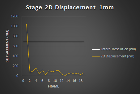

This experiment shows a significant initial displacement between Frame 0 and Frame 1, ranging from 1000 nm to 400 nm, which decreases to 70 nm by Frame 2. To quantify this variation, calculate the dispersion for each displacement using the formula: Dispersion = StandardDeviation(Displacement). Report the results in a table.
| Traveled Distance (mm) | 0 mm | 1 mm | 10 mm |
| X Dispersion (nm) | 4 | 188 | 121 |
| Y Dispersion (nm) | 4 | 141 | 48 |
| Z Dispersion (nm) | 10 | 34 | 53 |
| Repositioning Dispersion 3D (nm) | 6 | 227 | 91 |
| Repositioning Dispersion 2D (nm) | 2 | 226 | 90 |
Conclusion
Further Investigation
We observed a significant shift in the first frame, which was unexpected and invites further investigation. These variables can affect repositioning dispersion: i) Traveled distance, ii) Speed, iii) Acceleration, iv) Time, and v) Environment. We decided to test the first three.
Methodology
Processing
This experimental protocol generated a substantial number of images. To process them automatically in ImageJ/FIJI using the TrackMate plugin, we use the following script Stage Repositioning with Batch TrackMate-v7.py
This script automates the process of detecting and tracking spots using the TrackMate plugin for ImageJ/FIJI. To use it:
- Drop the script into the FIJI toolbar and click Run.
From v7, the FIJI script performs all the necessary tasks.
Prior v7, it was generating a CSV file for each image, which can be aggregated for further analysis using the accompanying R script, Process Stage Repositioning Results.R. This R script processes all CSV files in a selected folder and save the file as Stage-Repositioning_Merged-Data.csv in an "Output" folder on the user desktop for streamlined data analysis.
This R code automates the processing of multiple CSV files containing spot tracking data.
This script generate a single CSV File that can be further processed and summarized with a pivot table as shown in the following spreadsheet Stage-Repositioning_Template.xlsx
Using the first frame as a reference we can plot the average XYZ position for each frame.

As observed earlier, there is a significant displacement between Frame 0 and Frame 1, particularly along the X-axis. For this analysis, we will exclude the first two frames and focus on the variables of interest: (i) Traveled distance, (ii) Speed, and (iii) Acceleration and will come back to the initial shift later.
Repositioning Dispersion: Impact of Traveled Distance
Results
Plot the 2D displacement versus the frame number for each condition of traveled distance.

The data looks good now with the two first frames ignored. Now, we can calculate the average of the standard deviation of the 2D displacement and plot these values against the traveled distance..

We observe a power-law relationship, described by the equation: Repositioning Dispersion = 8.2 x Traveled Distance^0.2473
| Traveled Distance (um) | Repositioning Dispersion (nm) |
| 0 | 4 |
| 1 | 6 |
| 10 | 20 |
| 100 | 19 |
| 1000 | 76 |
| 10000 | 56 |
| 30000 | 107 |

Conclusion
Repositioning Dispersion: Impact of Speed and Acceleration
Results
Generate a plot of the 2D displacement as a function of frame number for each combination of Speed and Acceleration conditions. This visualization will help assess the relationship between displacement and time across the different experimental settings.

As noted earlier, there is a significant displacement between Frame 0 and Frame 1, particularly along the X-axis (600 nm) and, to a lesser extent, the Y-axis (280 nm). To refine our analysis, we will exclude the first two frames and focus on the key variables of interest: (i) Speed and (ii) Acceleration. To better understand the system's behavior, we will visualize the average standard deviation of the 2D displacement for each combination of Speed and Acceleration conditions.


Our observations indicate that both Acceleration and Speed contribute to an increase in 2D repositioning dispersion. However, a two-way ANOVA reveals that only Speed has a statistically significant effect on 2D repositioning dispersion. Post-hoc analysis further demonstrates that the dispersion for the Speed-Fast, Acc-High condition is significantly greater than that of the Speed-Low, Acc-Low condition.
| 2D Repositioning Dispersion (nm) | |
| Speed-Slow Acc-Low | 32 |
| Speed-Slow Acc-High | 49 |
| Speed-Fast Acc-Low | 54 |
| Speed-Fast Acc-High | 78 |
Conclusion
What about the initial shift ?
Right, I almost forgot about that. See below.
Results
Ploting the 3D displacement for each tested conditions from the preivous data.


We observe a single floating point that corresponds to the displacement between Frame 0 and Frame 1. This leads me to hypothesize that the discrepancy may be related to the stage's dual motors, each controlling a separate axis (X and Y). Each motor operates in two directions (Positive and Negative). Since the shift occurs only at the first frame, this likely relates to how the experiment is initiated.
To explore this further, I decided to test whether these variables significantly impact the repositioning. We followed the XYZ repositioning dispersion protocol, testing the following parameters:
- Distance: 1000 µm
- Speed: 100%
- Acceleration: 100%
- Axis: X, Y, XY
- Starting Point: Centered (on target), Positive (shifted positively from the reference position), Negative (shifted negatively from the reference position)
- For each condition, three datasets were acquired.
Data Stage-Repositining_Diagnostic-Data.xlsx was processed as mentioned before and we ploted the 2D displacement function of the frame for each condition.

When moving along the X-axis only, we observe a shift in displacement when the starting position is either centered or positively shifted, but no shift occurs when the starting position is negatively shifted. This suggests that the behavior of the stage’s motor or the initialization of the experiment may be affected by the direction of the shift relative to the reference position, specifically when moving in the positive direction.

When moving along the Y-axis only, we observe a shift in displacement when the starting position is positively shifted, but no shift occurs when the starting position is either centered or negatively shifted. This indicates that the stage's motor behavior or initialization may be influenced by the direction of the shift, particularly when starting from a positive offset relative to the reference position.

When moving along both the X and Y axes simultaneously, a shift is observed when the starting position is centered. This shift becomes more pronounced when the starting position is positively shifted in any combination of the X and Y axes (+X+Y, +X-Y, -X+Y). However, the shift is reduced when the starting position is negatively shifted along both axes.
Conclusion
Channel Co-Alignment
Channel co-alignment or co-registration refers to the process of aligning image data collected from multiple channels. This ensures that signals originating from the same location in the sample are correctly overlaid. This process is essential in multi-channel imaging to maintain spatial accuracy and avoid misinterpretation of co-localized signals. For a comprehensive guide on Channel Co-Registration, refer to the Chromatic aberration and Co-Registration the QuaRep Working Group 04.
Acquisition protocol
Processing
Results
The following spreadsheet provides a dataset that can be manipulated with a pivot table to generate informative graphs and statistics Channel_Co-registration_Template.xlsx.
Metrics
- The Nyquist ratio evaluates how closely the images align with the Nyquist sampling criterion. It is calculated as: Nyquist Ratio = Pixel Dimension / Nyquist Dimension
- A ratio of 1 indicates that the image acquisition complies with the Nyquist criterion.
- A ratio above 1 signifies that the pixel dimensions of the image exceed the Nyquist criterion.
- A ratio below 1 is the desired outcome, as it ensures proper sampling.
- The Co-Registration Ratios measure the spatial alignment between two channels by comparing the distance between the centers of corresponding beads in both channels to a reference distance. The reference distance is defined as the size of the fitted ellipse around the bead in the first channel.
- A ratio of 1 means the center of the bead in the second channel is located on the edge of the ellipse fitted around the bead in the first channel.
- A ratio above 1 indicates the center of the bead in the second channel lies outside the ellipse around the first channel's bead center.
- A ratio below 1 is the desired outcome, indicating that the center of the bead in the second channel is within a range smaller than the system's 3D resolution.
This method is the approach used in the MetroloJ QC Channel Co-Registration function.
Let's look at the 3D Colocalization Ratio for all pairs of channels.

For the 2x Objective we see that the 3D Colocalization Ratio is above 1 for the DAPI x GFP and DAPI x Cy5 pairs. This indicates that the chromatic shift is higher than the effective resolution of the system. Correction should be applied to images after acquisition. It somethimes possible to correct it before acquisition directly in the acquisition software. The correction values are provided by the Pixel Shift tables. Values highlighted correspond to a 3D Colocalization Ratio above 1.

These results shows a widefield instrument using a quadband pass filter: A single cube filtering 4 wavelengths. This instrument also possess individual filter cubes. Obviously the Colocalization Ratio are higher because of the mechanical shift induced by the filter turret.

With the corresponding Pixel Shift Table


Why should you care? Well when you are acquiring a multi-channel image you might see a significant shift between the two channels. This is particularly true for the combination of DAPI and Cy3 channels with the 10x Objective.


Report the Pixel Shift Table For each objective and each filter combination. This table can (should) be used to correct a multi-channel image by displacing the Channel 2 relative to the Channel 1 by the XYZ pixel coordinates indicated.
| Channel_2 | ||||||
| Objective | Channel_1 | Axis | DAPI | GFP | Cy3 | Cy5 |
| 2x | DAPI | X | 0.89 | -0.14 | -0.35 | |
| Y | 0.19 | 1.63 | 2.00 | |||
| Z | 0.89 | 3.67 | 1.58 | |||
| GFP | X | -0.89 | -1.04 | -1.25 | ||
| Y | -0.19 | 1.44 | 1.81 | |||
| Z | -0.89 | 2.78 | 0.70 | |||
| Cy3 | X | 0.14 | 1.04 | -0.21 | ||
| Y | -1.63 | -1.44 | 0.37 | |||
| Z | -3.67 | -2.78 | -2.08 | |||
| Cy5 | X | 0.35 | 1.25 | 0.21 | ||
| Y | -2.00 | -1.81 | -0.37 | |||
| Z | -1.58 | -0.70 | 2.08 | |||
| 10x | DAPI | X | 0.46 | -0.85 | -1.16 | |
| Y | 0.50 | 1.79 | 2.27 | |||
| Z | 4.22 | 4.44 | 1.91 | |||
| GFP | X | -0.46 | -1.31 | -1.61 | ||
| Y | -0.50 | 1.29 | 1.77 | |||
| Z | -4.22 | 0.22 | -2.31 | |||
| Cy3 | X | 0.85 | 1.31 | -0.30 | ||
| Y | -1.79 | -1.29 | 0.48 | |||
| Z | -4.44 | -0.22 | -2.53 | |||
| Cy5 | X | 1.16 | 1.61 | 0.30 | ||
| Y | -2.27 | -1.77 | -0.48 | |||
| Z | -1.91 | 2.31 | 2.53 | |||
| 20x | DAPI | X | 0.58 | -0.77 | -1.06 | |
| Y | 0.13 | 1.23 | 1.54 | |||
| Z | 3.31 | 3.95 | 2.09 | |||
| GFP | X | -0.58 | -1.35 | -1.64 | ||
| Y | -0.13 | 1.10 | 1.41 | |||
| Z | -3.31 | 0.64 | -1.22 | |||
| Cy3 | X | 0.77 | 1.35 | -0.29 | ||
| Y | -1.23 | -1.10 | 0.31 | |||
| Z | -3.95 | -0.64 | -1.86 | |||
| Cy5 | X | 1.06 | 1.64 | 0.29 | ||
| Y | -1.54 | -1.41 | -0.31 | |||
| Z | -2.09 | 1.22 | 1.86 | |||
| 63x | DAPI | X | 0.13 | -1.52 | -2.03 | |
| Y | 0.13 | 1.19 | 1.66 | |||
| Z | 0.79 | 1.31 | 0.93 | |||
| GFP | X | -0.13 | -1.65 | -2.16 | ||
| Y | -0.13 | 1.06 | 1.53 | |||
| Z | -0.79 | 0.52 | 0.13 | |||
| Cy3 | X | 1.52 | 1.65 | -0.51 | ||
| Y | -1.19 | -1.06 | 0.47 | |||
| Z | -1.31 | -0.52 | -0.39 | |||
| Cy5 | X | 2.06 | 2.22 | 0.51 | ||
| Y | -1.73 | -1.59 | -0.47 | |||
| Z | -0.92 | -0.12 | 0.39 | |||
Conclusion
Legend (Wait for it)...
For a comprehensive guide on Detectors, refer to the Detector Performances of the QuaRep Working Group 02.
Acquisition protocol
Results
Conclusion
Legend (Wait for it...) dary
For a comprehensive guide on Lateral and Axial Resolution, refer to the Lateral and Axial Resolution of the QuaRep Working Group 05.
Acquisition protocol
Results
Conclusion
A microscope can capture a defined area of a sample. This area is called Field-of-View (FOV) and depends on the optical configuration and microscope acquisition device. This is a limiting feature of microscopy. To be able to observe with a higher resolution the total visualized area is reduced. This can be an issue when trying to visualize feature that are bigger than the FOV.
One way to deal with this issue is to acquire multiple images and stitch them together after acquisition. Instead of acquiring adjacent FOV it is best to have partially overlapping regions. These regions will help to stitch images together.
While many softwares provide proprietary stitching solution we will focus here on the free and versatile plugin for ImageJ named Grid Collection Stitching.
Developed by Stephan Preibisch, this plugin is also part of FIJI distribution of ImageJ.
Stitching process
Stitching usually occurs in 3 steps:
- The first is the "layout" which finds the adjacent images for each given image. This step approximatively place the images in relation to each other.
- The second step finely transform (rotation, translation) one image to the adjacent ones. It matches detected features in one image to the same feature in the adjacent image
- The last step blends the images so the results appears smooth
Layout
Three pieces of information can be used to define the layout.
1. Images metadata
Modern microscopes use motorized stages to move the sample in X and Y. These coordinates can be stored in the image metadata and used during stitching. Knowing the approximate position of each tile greatly help stitching as you just have to compute the fine matching between the different images.
2. Tiles configuration and acquisition order
if you have 25 images (Image 1, Image 2,....) and know that it comes from a 5 x 5 acquisition from the top left to the bottom righ, by row from left to right; then you can quickly place your images to their approximate positions. Sometimes the tile configuration is directly saved into the file names (Image X1Y1, Image X2Y1 etc.), this can also be used to define the approximate tile layout
3. Images themselves
The data in the image can also be used to define the layout. It requires computing power as it usually parse all possible pairwise combination and compute a correlation coefficient. It then matches images with highest correlation.
Transformation
Once the layout is defined, the images need to be finely adjusted one to another. Because microscopes are not perfect some translation and rotation can be used to finely match identified features in adjacent images. To do this images are usually acquired with a 10 to 20% overlapping region. This region will be used to finely match adjacent images.
Blending
A blending can be applied to the overlapping region to ensure a smooth tiled result.
Protocol
- Open up FIJI
- Open the Grid/Collection stitching plugin Menu Plugins>Stitching>Grid/Collection stitching
Your files are saved under Tile_x001_y001.tif, you know the grid size and the percentage overlap
- Type: Filename defined position
- Order: Defined by filename
- Click OK
- Indicate the grid size (for example 5x5 if you have 25 images)
- Under directory click Browse
- Select the folder containing your files
- Click Choose
- Under file names for tiles Tile_x{xxx}_y{yyy}.tif
Several options are available I recommend using the following:
- Add tiles as ROIs (to check tiling quality
- Compute Overlap
- Display fusion
Your files are saved under Tile_001.tif, you know the grid size, the acquisition order and the percentage overlap
- Type: Grid: Column by column
- Order: Down & Right
- Click OK
- Indicate the grid size (for example 5x5 if you have 25 images)
- Under directory click Browse
- Select the folder containing your files
- Click Choose
- Under file names for tiles Tile_{iii}.tif
Several options are available I recommend using the following:
- Add tiles as ROIs (to check tiling quality
- Compute Overlap
- Display fusion
- Subixel accuracy
Your are capturing images with a manual stage. If you read this before the acquisition I would suggest to acquire your tiles using a given size and scheme (for example 3x3 snake horizontal right). This will allow to use the process above (except Type Grid: Snake by rows). Make sure to have some overlap between images to be able to finely place them. Since you are probably reading this after your acquisition you would have file saved as Tile_001.tif... but you do not know the grid size or the acquisition order nor the percentage overlap
- Type: Unknown position
- Order: All files in Directory
- Click OK
- Under directory click Browse
- Select the folder containing your files
- Check Confirm files
Several options are available I recommend using the following:
- Add tiles as ROIs (to check tiling quality
- Ignore Z stage position
- Subpixel accuracy
- Display fusion
- Computation parameters: Save computation time
If you choose Type: Grid the plugin except sequential continuous files i i+1 etc...
If you choose Positions from File the plugin expect one single file multiseries file. To Combine several files into one single T series, open the images individually or all together Then combine them as a stack
Image>Stacks>Images to Stack
Check use tiltes as labels
then convert the Stack to a T serie
Image>Hyperstacks>Stacks to Hyperstacks
Slices (z)=1 Frames (t)=number that was in z and you have replaced by 1
In my experience proprietary softwares do not encode X and Y values in the metadata properly so this method is not often used
Type: Positions from file
Use this is you want to use the image metadata to define the tile positions. This only works if you have one single input file with all the tiles inside. In my experience this works when the file issaved under the acquisition software proprietary format.
You can also use this type of stitching if you have an additional text files defining the position of each image. You can also create this file yourself
# Define the number of dimensions we are working on
dim = 3
# Define the image coordinates (in pixels)
img_01.tif; ; (0.0, 0.0, 0.0)
img_05.tif; ; (409.0, 0.0, 0.0)
img_10.tif; ; (0.0, 409.0, 0.0)
img_15.tif; ; (409.0, 409.0, 0.0)
img_20.tif; ; (0.0, 818.0, 0.0)
img_25.tif; ; (409.0, 818.0, 0.0)
Notes
The higher the overlap the more computing power required.
Percentage overlap is approximate. Starts low and increase until result is satisfying
It is much easier to stitch when the layout is known.
It is much easier to stitch images when there are many visible features: slide of tissue is easier than sparse cell culture; bright field images are easier than fluorescence images
Renaming your files
You can easily rename files on a mac using Automator.
On a PC you can use Bulk Rename Utility
More information
https://imagej.net/plugins/image-stitching
Introduction
Microscopy is an approximation of reality. The point spread function is the better example of this: A single point will appear as a blurry ellipse using photonic microscopy. This transformation depends on the optical components which varies with time.
Quality control monitors this transformation over time.
Download MetroloJ QC from GitHub - MontpellierRessourcesImagerie/MetroloJ_QC
Download iText Library v 5.5.13 from https://repo1.maven.org/maven2/com/itextpdf/itextpdf/5.5.13.2/itextpdf-5.5.13.2.jar
Download ImageJ Download (imagej.net) or FIJI Fiji Downloads (imagej.net)
Open ImageJ or FIJI
Install MetroloJ QC and iTextPDF by dropping the .jar file into ImageJ status bar
Start up the microscope
Follow the set up procedure (load the test sample and focus with the lowest magnification objective).
Adjust to obtain a Kholer illumination
Remove the sample from the microscope
Nikon Ti2 without occular a shadow appears on the upper left corner of the FOV
Take a BF image for Widefield illumination Homogeneity
Analyze the image using MetroloJ QC and Check centering accuracy and total homogeneity
4x

Here the centering is off to the left side and the intensity is falling below 30%.
replace the illumination arm by the application screenlight

removing the objective:

If image is similar then the issue comes from the detection side.
Test all items on the detection path: Objective, filter cubes, lightpath selector, camera
Objective 20x-075

It improve the hopmogeneity but centering is still off
60x1.4 gives a perfect homogeneity

Repeat for each objective
Change objective
Adjust Kholer
Take a BF image for Widefield illumination Homogeneity
If illumination is not homogeneous then
Conclusion: Camera may be re-aligned to obtain an homogenous illumination in bright field.
5408nm laser line not working used for YFP. Laser is shining outside the fiber but not reachingh the objective. Has the cube been changed?
Immersion Oil
Very important component. Mostly used for oil immersion objectives, the refractive index should match the RI of glass from the coverslip and the objectives used. Different types or grades are available A (Low viscosity), B (high viscosity), N, F, FF (for fluorescence) etc... as well as different viscosity. Because the refractive index (and viscosity) vary with the temperature you should buy immersion oil matching the room temperature. Usually 23C but you could also need 30C and 37C.
To date Cargille provide the best options
Cargille
- Cargille Immersion Oil type FF #16212, 16 oz (473mL), 94$, 0.2$/mL RI=1.48
- Cargille Immersion Oil type HF #16245, 16 oz (473mL), 94$, 0.2$/mL RI=1.51
- Cargille Immersion Oil type LDF #16241, 16 oz (473mL), 94$, 0.2$/mL RI = 1.51
Extremely low fluorescence is achieved by Type LDF and Type HF. Type FF is virtually fluorescence-free, though not ISO compliant. Type HF is slightly more fluorescent than Type LDF, but is halogen-free.
Thorlabs
- MOIL-30 Olympus Type F, 30mL, $84, 2.8$/mL
- MOIL-20LN Leica Type N, 20mL, $75, 3.75$/mL
- OILCL30 Cargille Type LDF, 30mL, $28, 1.1$/mL RI=1.51
- MOIL-10LF Leica Type F, 10mL, $59, 5.9$/mL
https://www.thorlabs.com/newgrouppage9.cfm?objectgroup_id=5381
Zeiss
- Immersion Oil Immersol 518F 20mL RI:1.518 t 23C - 444960-0000-000 Prices varie from 56$ to 156$ (and even 580$/each); 2.8$ to 7.8$/mL https://www.micro-shop.zeiss.com/en/ca/accessories/consumables
- 30C 444970-9000-000
- 37C 444970-9010-000
Edmund Optics
- Olympus Low fluorescence immersion oil type F, #86-834, 30mL, 113$; 3.8$/mL https://www.edmundoptics.ca/p/olympus-low-auto-fluorescence-immersion-oil/29243/
Lens Cleaner
Use a lens cleaner to clean objective lenses from oil.
Tiffen
Tiffen is a great product designed for camera lenses but it works great for microscope optics as well
- Tiffen Lens Cleaner 16oz (472mL) #EK1463728T 14$ 3cts/mL https://tiffen.com/products/tiffen-lens-cleaner-16oz
Edmund Optics
- Lens Cleaner #54-828 (8oz, 236mL) 14$; 6 cts/mL
- Purosol #57-727 (4oz, 115mL), 29$, 25 cts/mL
Zeiss, Nikon, Olympus, Leica
- Home made recipe: 85% n-hexane analytical grade, 15% isopropanol analytical grade
Lens tissue
Edmund Optics
- Lens Tissue #60-375 500 sheets 36$ 7cts/sheet
Thorlabs
- Lens Tissue #MC-50E 1250 sheets 93$ 7.6cts/sheet
Tiffen
- Lens Tissue #EK1546027T 250 sheets 112$ 44cts/sheet
Liquid light guides
Excelitas
- 3mm core diameter, 1.5m length sold by Digikey #1601-805-00038-ND 682$
Thorlabs
- 3mm core diameter, 1.2m length #LLG03-4H 410$
- 3mm core diameter, 1.8m length #LLG03-6H 490$
Edmund Optics
- 3 mm core diameter, 1.8m length #53-689 3mm 700$
- Adapters available #66-905
Microscope world
- Liquid Light Guide 3mm core diameter, 1.5m length #805-00038 445$
Bulbs
AVH Technologies
HXP R 120W/45C 780$
OSRAM
XP R 120 W/45 #69119
Others consumables
- Cotton swab
- Absorbent polyester swabs for cleaning optical components, Alpha, Clean Foam or Absorbond series TX743B) from www.texwipe.com
- Rubber Blower GTAA 1900 from Giottos www.giottos.com
Let's say you have many images taken the same way from two different samples: One Control group and One test group.
What will/should you do to analyse them?
The first thing I would do will be to open a random pair of image (one from the control and one from the test) and have a look at them...
Control Test


Then I would normalize the brightness and contrast for each channel and across images to make the display settings the same for both images.
Then I would look at each channel individually and use a LUT Fire to have better appreciate the intensities.
Finally I will use the syncrhonize Windows features to navigate the two images at the same time
ImageJ>Windows>Synchronize Windows
ou dans une macro
run("Synchronize Windows");
Control Ch1 Test Ch1

Control Ch2 Test Ch2

To my eyes the Ch1 and Ch2 are slighly brighter in the Test conditions.
Here we can't compare Ch1 to Ch2 because the range of display are not the same. It seems than Ch2 is much weaker than Ch1 but it is actually not accurate. The best way to sort this is to add a calibration bar to each channel ImageJ>Tools>Calibration Bar. The calibration bar is non-destructive as it will be added to the overlay. To "print" it on the image you can flatten it on the image ImageJ>Image>Overlay>Flatten.
Control Ch1 Control Ch2


If you apply the same display to Ch1 and Ch2 then you can see that Ch1 overall more intense while Ch2 has few very strong spots.
Control Ch1 Control Ch2 with same display than Ch1

Looking more closely
In Ch1 we can see that there is some low level intensity and a high level circular foci whereas in Ch2 there is a bean shaped structure. In the example below the Foci seems stronger in the control than the Test condition.
Control Ch1 Test Ch1


Control Ch2 Test Ch2


But we need obviously to do some quantification to confirm or infirm these first observations.
The first way to address it would be in a bulk fashion: By measuring the mean intensity for example for all the images.
If all works fine you should have a CSV file you can open with your favorite spreadsheet applications. This table should give one line per image and all available measurements for the whole image and for each channel of the image. Of course some measurements will be all the same because the images were taken in the same way.
What to do with the file? Explore the data and see if there is any relevant information.
My view would be to use a short script in R to plot all the data and to some basic statistics
This should give you a pdf file with one plot per page. You can scroll it and look at the data. p-values from t-test are indicated on the graphs. As you can see below the mean intensity in both Ch1 and Ch2 are higher in the test than the control. What does it mean?
It means than the average pixel intensity is higher in the test conditions than the control condition.
Other values that are significantly different:
- Mean Intensity Ch1 and Ch2 (Control<Test)
- Maximum Intensity of Ch1 (Control>Test) Brightest value in the image
- Integrated Intensity of Ch1 and Ch2(Control<Test) It is equal to the Mean x Area
- Median Ch1 and Ch2 (Control<Test)
- Skew of Ch1 (Control>Test): The third order moment about the mean. Relate to the distribution of intensities. If=0 then intensities are symmetrically distributed around the mean. if<0 then distribution is asymmetric to the Left of the mean (lower intensities), if>0 then it is to the right (higher intensities).
- Raw Integrated Intensities of Ch1 and Ch2 (Control<Test) Sum of all pixel intensities
Now we start to have some results and statistically relevant information about the data. The test condition have a higher mean intensity (integrated intensity, median and raw integrated intensities are all showing the same result) for both Ch1 and Ch2. This is surprising because I had the opposite impression while looking at the image with normalized intensities and LUT fire applied (see above). Another surprising result is the fact that Control images have a higher maximum intensity than Test images but only for Ch1. This is clearly seen in the picture above.
One thing that can explain these results is that the number of cells can be different in the control vs the test images. If there are more cells in one condition then there are more pixels stained (and less background) and the mean intensity would be higher not because the signal itself is higher in each cell but because there are more cell...
To solve this we need to count the number of cells per image. This can be done manually or using segmentation based of intensity.
Looking at the image it seems that Ch1 is a good candidate to segment each cell.
This macro starts to be a bit long but to summarize here are the steps:
- Open each image
- Remove the offset from the camera (500 GV) and apply a rolling ball background subtraction
- Create a RGB composite regrouping both channels
- Convert this RGB to a 16-bit image
- Threshold the RGB image using the Otsu alogrythm
- Process the binary to improve detection (Open, Dilate, Fill Hole)
- Analyze particles to detect cells with size=2-12 circularity=0.60-1.00
- Add the results to the ROI manager
- Save the Mask for the control of segmentation
- Save an RGB image with the detection overlay as a control for the good detection
- Save the ROIs
- Use the ROIs to collect all measurements available and save the result as a csv
- Save the image with the background removed
- Crop each ROI from the image with the Background removed to isloate each cell
Few notes:
The camera offset is a value the camera adds to avoid having negative value due to noise. The best way to measure it is to take a dark image and have the mean intensity of the image. If you don't have that in hand you can choose a value sligly lower than the lowest pixel value found in your images.
The rolling ball background subtraction is powerfull tool to help with the segmentation
The values for the Analyze particles detection are the tricky part here. How I choose them? I use the thresholded image (binary) and I select the average guy: the spot that looks like all the others. I use the wand tool to create a selection and then I do Analyze>Measure This will give me a good estimate of the size (area) and the circularity. Then I select the tall/skinny and the short/not so skinny guys: I use again the wand tool to select the spots that would be my upper and lower limits. This will give me the range of spot size (area) and circularity. This is really a critical step that should be performed by hand prior running the script. You should do this on few different images to make sure the values are good enough to account for the variability you will encounter.
Now it is time to check that the job was done properly.
Looking at the control Images the detection isn't bad at all.


The only thing missing are the individual green foci seen below. Those cells look different as the FOci is very strong but there is not much fluorescence elsewhere (no diffuse green and no red). I might discuss with the scientist to see if it is OK to ignore them. If not I would need to change the threshold values and the detection parameters but let's say it is fine for now.

So now you should have a list of files (images, ROIs, and CSV files). We will focus on the CSV files has they contain the number of cells we are looking for and a lot more information we can also use.
We will reuse the previous R script but will add a little part to merge all the CSV files from the input folder.
This script will save the merged data in a single csv file. Usign your favourite spreadsheet manager you will be able to create a table and summarize the data with a pivot table to get the number of cells per group.
| Control | Test |
| 1225 | 1360 |
There are slighly more cells in the test than in the control. If we look at the number of detected cells per image we can confirm that there are more cells in the test conditions than in the control conditions. There are two images that have less celss than others in the control. We can go back to the detection to check those.

Looking at the detection images we can confirm that the two images from the control have less cells, so it is not a detection issue.


Together these results show that there is no more cells in one condition than the other.
On avera between 60 and 65 cells are detected by image with a total of 1200 cells per condition detected.
Then we can look at the graphs and look for what is statistically different, here is the short list
- Area Test>Control
- Mean Ch2 Test>Control
- Min Ch2 Test>Control
- Max Ch1 Control>Test
- Max Ch2 Test>Control
- Perimeter Test>Control
- Width and Height Test>Control
- Major and Minor Axis Test>Control
- Feret Test>Control
- Integrated Density Ch1 et Ch2 Test>Control
- Skew et Kurt Ch1 Control>Test
- Raw Integrated density of Ch2 Test>Control
- Roundness Control>Test
Looking at p-values (statistical significance) is good approach but it is not enough. We should also look at the biological significance of the numbers. For example the roundess is statiscially different between the control and test but this difference is really small. What does it mean biologically that the test cells are a tiny bit less circular. In this specific case : nothing much. So we can safely forget about it to focus on more important things.
This can easily be done since we have generated a CSV file gathering all the data Detected-Cells_All-Measurements.csv
Then for all the variables that are statically different between control and test groups we can have a closer look at the data.
- Area Control 5.03um2 ; Test 5.35um2 p-value = 1.7e−07
This is a relatively small increase 6%. If we bring this back to the diameter it is even smaller 3% increase. Yet the most relevant value in my view is the volume because cells are spheres in the real life. This increase is about a 10% increase in the cell volume. This is relevant information. Cells in the Test conditions are 10% bigger than in the control condition. - Mean Ch2 Control 1078 GV; Test 1197 GV p-value < 2.2e−16
This means that the bean shape structure labelled by Ch2 is 10% brighter in the test cells than in the controls. Yet the segmentation was performed on the full cell using Ch1 as a proxy. This result prompt for a segmentation based on Ch2. Are the bean shaped bigger or brighter? - Min Ch2 Control 198 GV; Test 213 GV p-value 1e−05
The difference in the minimum of Ch2 represent about 7.5% increase. If the minimum is higher it suggests that there is a global increase in the fluorescent of Ch2 and not a redistribution (ie clusterization). The segmentation on the Ch2 might sort out which option is really occurring - Max Ch1 Control 10111 GV; Test 8393 GV p-value < 2.2e−16
This difference represent a 17% decrease of the maximum intensity of Ch1. If we remember Ch1 has two fluorescent levels, low within the nuclei and an intense foci. Here the maximum represent the Foci only. So we can conclude that the Foci are less intense in the test compare to the control. - Max Ch2 Control 3522 GV; Test 3761 GV p-value = 0.00035
Here we have the opposite situation where in the bean shape structure the maximum intensity is higher in the test condition than the control - Perimeter Control 8.45um ; Test 8.74um p-value = 1.7e−08
Here we have another measurement about the size of the detected cells. Using the area we can estimate about a 3.1% perimeter increase. Here the increase is about 3.5%. This is consistant meaning the increase in area and perimeter are about the same. - Width and Height Control 2.49um; Test 2.57um p-value = 8e−07
Again here another measurement of the size of the detected cells which are larger in the test than the control - Major and Minor axis length Control 2.73um; Test 2.84um p-value = 2.7e−10
Similar to above excepted that instead of measuring the width and heigh of a rectangle around the cell it is an ellipse fitting the cell. In my view this would be more relevant variable than the previous one but since all data converge to slightly larger cells in the test than the control we can focus on the most interesting ones (area or perimeter) - Feret Control 2.95um; Test 3.05um p-value = 5.1e−10
This is the maximum distance between two points of the detected cells. It relates to the shape of the cell - Integrated Density Ch1 Control 11296 GV; Test 11886 GV p-value
This is the product of area and mean intensity. We know that the area is larger but not the mean intensity. Yet the integrated density of Ch1 is sligtlhy larger (5%) in test vs control. - Integrated Density Ch2 Control 5570 GV; Test 6548 p-value < 2.2e−16
Here we have a 17% increase which represent the combination of increase of cell size and mean intensity of Ch2 - Skew of Ch1 Control 2.47; Test 1.77 p-value < 2.2e−16
The skewness refers to the asymmetrical shape of the distribution of the intensities. Since values are above 0 it means that the distribution is skewed towards the higher intensities. Since this number is lower in the test cells, it means that the distribution of Ch1 intensity is less asymmetric. This can be easily explained by looking at Ch1 which has a low intensity within the nuclei and a strong foci. The foci high intensities provides a higher skew number. Since the skew is less closer to 0 in test conditions this could mean that the foci is less intense or that the fluorescence of Ch1 is more evenly distributed. Since we don't have an increase nor a decrease of mean intensity in Ch1 it is likely that the fluorescence is more evenly distributed in the test condition Thant the control. In other words it seems that in the control conditions the foci is brighter by taking some of the low fluorescence that is present in the nuclei. In other words, it seems that the test conditions can't make very bright foci and that the Ch1 fluorescence is more evenly distributed. - Kurt of Ch1 Control 11.3; Test 7.24 p-value < 2.2e−16
The Kurt account for the flatness of the distribution. If Kurt=0 we have a normal distribution, if <0 it is flatter than normal; if >0 it is more peaked. In this case the data is very very peaked in both control and test. This is quite interesting especially when looking at the violin graphs below. In the control we can see 2 peaks one close to 0 and one close to 11. This means that there are two kinds of cells in the control condition, the one with a foci and the one with only low level distributed Ch1 fluorescence. In the test conditions the Kurt are entered and the two peaks are so close that they almost merged. - Raw Integrated density of Ch2 Control 313299 vs Test 368339; p-value < 2.2e−16
This is the sum of the pixel intensities. It is higher in the test cell than the control cell. This can be because the intensity is higher and/or the area is larger. In this case we have seen previously that the area is larger. Interestingly Raw intensity is higher for Ch2 but is the same for Ch1. - Roundness Control 0.84; Test 0.83 p-value = 0.0032
As said before even though the value is significant the difference here is minimal and we can easily go to focus on another
As we have seen here it seems that Ch1 and Ch2 have defined structrures that differs between the Control and test group. Our analysis looking at each cell does not provide enough detail on each structure. More specifically it can't discriminate between the low intensity Ch1 and the high intensity Foci. Also it looks at the overall fluorescence of Ch2 in the cell while we can clearly identify a bean shape structure. The next step would be to segment the images in 3 ways: high Ch1 intensities would correspond the the foci, high Ch2 intensities would correspond to the bean shape structure and low Ch1 intensities (all Ch1 intensities but excluding the high intensities from the Foci) would relate to the overall nuclei
What are the parameters to choose a good objective
What is the strehl ratio?
Screw type
RMS (Royal Microscopical Society objective thread)
M25 (metric 25-millimeter objective thread)
M32 (metric 32-millimeter objective thread).
Less common or older
M27 x0.75
M27x1.0
Working distance
Immersion
Numerical aperture
Optical Correction
Transittance
Others
Tubelength
Adjustment
I get often questions about how to write the Marterial and Method section of a manuscript including microscopy data. The diversity of technologies and applications in the field of microscopy may be complicated for some users and help of a microscopy specialist is often required.
Here I would like to present a usefull tool called MicCheck that provides a checklist of what to include in the material and method section of a manuscript including microscopy data. MicCheck is a free tool to help you. It is described in details in the following article.
Montero Llopis, P., Senft, R.A., Ross-Elliott, T.J. et al. Best practices and tools for reporting reproducible fluorescence microscopy methods. Nat Methods 18, 1463–1476 (2021). https://doi.org/10.1038/s41592-021-01156-w
Received
Accepted
Published
Issue DateDecember 2021

What is photo-toxicity?
Under appropriate conditions of temperature (37°C), high humidity, and a controlled atmosphere (5% CO2), it is possible to grow cells in vitro. However, observing these cells under a microscope can have unintended effects. This situation is analogous to exposing yourself to sunlight: if the sunlight is too intense or the exposure lasts too long, you may suffer a sunburn. Similarly, cells can be affected by prolonged or intense light exposure during microscopy. While transmitted light (bright-field, phase-contrast, DIC) generally does not interfere with cell biology, fluorescence excitation light can cause significant phototoxic effects.

Healthy cells
What does phototoxicity look like?
Prolonged exposure to intense illumination can cause significant cellular damage, resulting in retraction, detachment, and eventual cell death. The example below demonstrates this process (click on the image to watch the movie).

Click on the image to see the movie
Cells subjected to 1 second of 59 mW, 395 nm light and 1 s 750 mW 550nm every 5 minutes. The total duration of the movie is approximately 8 hours.
 Click on the image to see the movie
Cells subjected to 1 second of 70 mW, 550 nm light every 5 minutes. The total duration of the movie is approximately 3 hours, during which the cells gradually retract, detach, and eventually die
How can I identify if phototoxicity has occurred?
The most effective way to detect phototoxicity is to capture a larger field-of-view image after your acquisition. Since phototoxicity is confined to the illuminated area, comparing adjacent non-illuminated cells with those in the exposed region offers a good—though not perfect—approach.
By stepping back, you can observe that the damage is limited to the illuminated area. However, it’s important to note that the recorded region may be smaller than the actual exposed area.
It’s also crucial to understand that this method is not a flawless control. A more ideal control would involve using a separate dish with cells maintained under identical conditions but without illumination. This is because, in the image above, we cannot definitively conclude whether the affected circular region has no impact on nearby cells. It’s possible that cell death in the illuminated region may release molecules that influence the surrounding cells. Therefore, the most reliable control would be a completely separate dish with unexposed cells.
Taking an overview

6 x 6 Tiles around the image area.
What are the important factors to consider when discussing phototoxicity?
Several key factors influence phototoxicity:
- Amount of light: Strong illumination causes more damage compared to dimmer light.
- Wavelength: The energy carried by light depends on its wavelength. Shorter wavelengths carry higher energy and tend to be more harmful.
- Illuminated area: Concentrating the same amount of light on a smaller area results in more localized damage.
- Duration of illumination: Prolonged exposure (e.g., 1 second vs. 10 ms) increases the risk of damage.
- Repetition of illumination: Frequent exposure (e.g., 10 ms pulses applied 20 times per minute) is more damaging than less frequent exposure (e.g., once per minute).
How can you detect phototoxicity?
Empirically, phototoxicity can be identified by observing cell behavior. If cells are not dividing, retracting, or detaching, it may indicate phototoxicity.
To assess phototoxicity:
- Acquire a larger field-of-view image of the recorded area to ensure no phototoxicity has occurred and to evaluate photobleaching.
- Use a power meter to measure the energy your cells are exposed to.
- Measure the power at the objective using your usual imaging settings.
- Record the value in mW (milliwatts = Joules/second).
- Divide this value by the field of view area (in cm²) to calculate the irradiance in mW/cm².
How to determine the maximum acceptable irradiance:
Finding an irradiance level that is stress-free for your cells is critical:
- Expose your cells continuously to a defined irradiance.
- Observe them over several hours. If they show no signs of phototoxicity, gradually increase the irradiance and repeat the observation.
- Identify the maximum continuous irradiance that does not cause damage.
Keep in mind that this value provides a baseline. Since most experiments do not involve continuous exposure, it is possible to exceed this threshold briefly. However, doing so may induce temporary stress in the cells. It is up to you to decide whether this level of stress is acceptable for your specific experiment and whether it might interfere with the biological processes you are studying.
Subtle example
 Click on the image to see the movie
Cells were imaged for 100ms with 70mW of 550nm light every 5 minutes. Cells are dividing faster than the effect of photo-toxicity that is occurring.
This is not a strictly a microscopy technic. It is more a method for sample preparation in which the sample is embedded in a Gel matrix which is digested and physically expended. Conventional microscopy acquisition is then applied to the expanded sample.
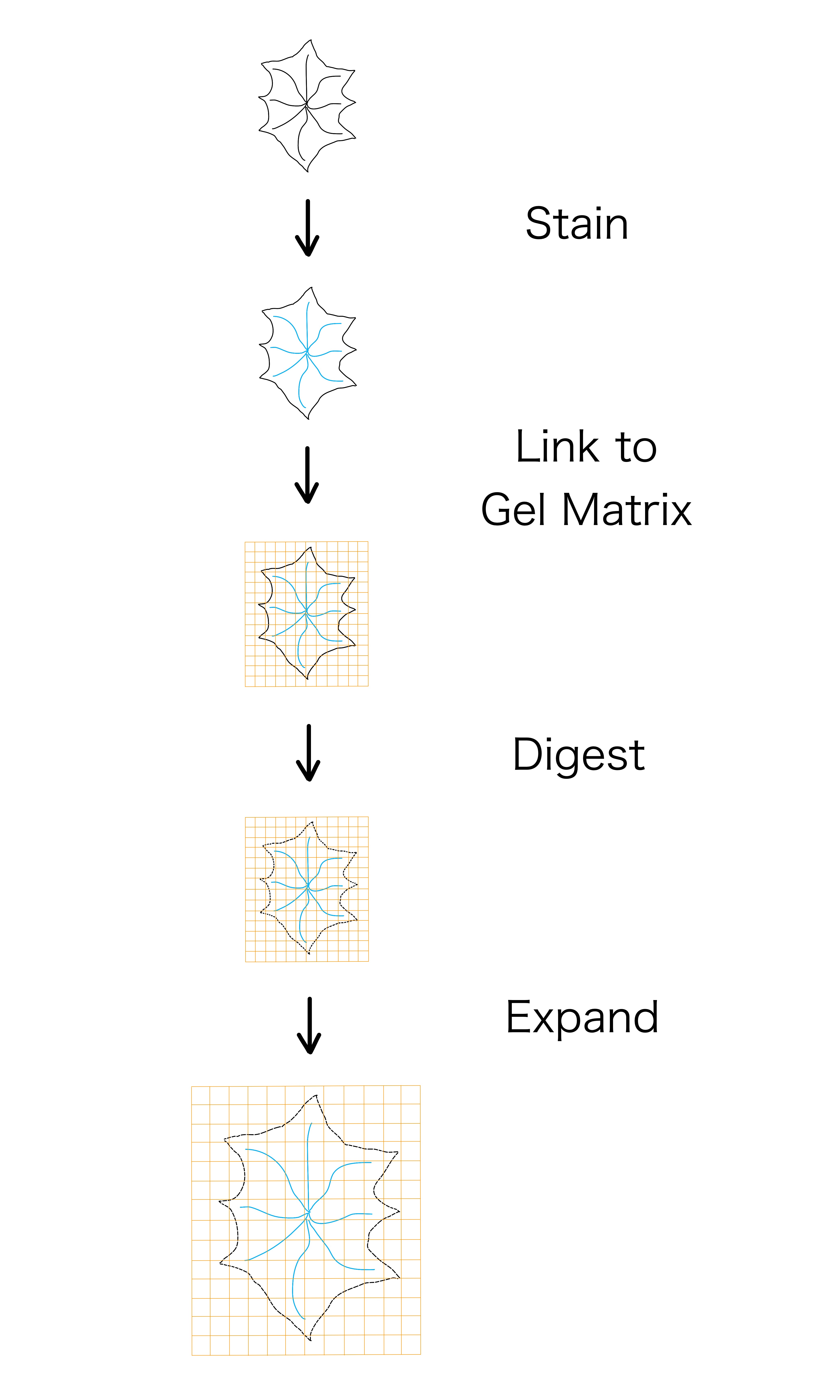
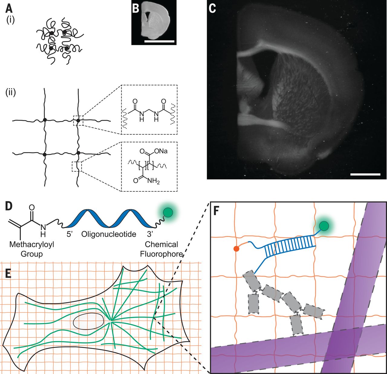
See
https://pubmed.ncbi.nlm.nih.gov/25592419/
https://en.wikipedia.org/wiki/Expansion_microscopy