
This page provides a practical guide for microscope quality control. By following the outlined steps, utilizing the provided template files, and running the included scripts, you will have everything needed to easily generate comprehensive report on your microscope's performance.
Equipment used
- Thorlabs Power Meter (PM400) and sensor (S170C)
- Thorlabs Fluorescent Slides (FSK5)
- TetraSpeck™ Fluorescent Microspheres Size Kit (mounted on slide) ThermoFisher (T14792)
Software used
- FIJI FIJI
- MetroloJ_QC Plugin for FIJI MetroloJ_QC
- iText Plugin for FIJI iText
- R R from the CRAN R Project
- I typically use the integrated development environment (IDE) for R RStudio
Please note that during quality control, you may, and likely will, encounter defects or unexpected behavior. This practical guide is not intended to assist with investigating or resolving these issues. With that said, we wish you the best of luck and are committed to providing support. Feel free to reach out to us at microscopie@cib.umontreal.ca
Illumination Warmup Kinetic
When starting light sources, they require time to reach a stable and steady state. This duration is referred to as the warm-up period. To ensure accurate performance, it is essential to record the warm-up kinetics at least once a year to precisely define this period.
Acquisition protocol
Results
Use the provided spreadsheet template, Illumination Warmup Kinetic_Template.xlsx, and fill in the orange cells to visualize your results. For each light source, plot the measured power output (in mW) against time to analyze the data.

Calculate the relative power using the formula: Relative Power = (Power / Max Power). Then, plot the Relative Power (%) against time to visualize the data.

We observe some variability in the power output for the 385 nm light source.
To assess the stability:
Define a Stability Duration Window:
Select a time period (e.g., 10 minutes) during which the power output should remain stable.Specify a Maximum Coefficient of Variation (CV) Threshold:
Determine an acceptable variability limit for the selected window (e.g., 0.01%).Calculate the Coefficient of Variation (CV):
Use the formula: CV = (Standard Deviation / Mean)
Compute the CV for the specified stability duration window.Visualize Stability:
Plot the calculated CV over time to analyze the stability of the power output.


We observe that the light sources stabilize quickly, within less than 10 minutes, while the 385 nm light source takes approximately 41 minutes to reach stability.
Report the results in a table
| 385nm | 475nm | 555nm | 630nm | |
| Stabilisation time (Max CV 0.01% for 10 min) | 41 | 3 | 3 | 8 |
| Stability Factor (%) Before Warmup | 99.7% | 99.9% | 100.0% | 100.0% |
| Stability Factor (%) After Warmup | 100.0% | 100.0% | 100.0% | 99.9% |
Selected Stability Duration Window (min): 10 min and Maximum Coefficient of Variation: 0.01%
Conclusion
Maximum Power Output
This measure assesses the maximum power output of each light source, considering both the quality of the light source and the components along the light path. Over time, we expect a gradual decrease in power output due to the aging of hardware, including the light source and other optical components. These measurements will also be used to track the performance of the light sources over their lifetime (see Long-Term Illumination Stability section).
Acquisition protocol
Results
Fill in the orange cells in the Maximum Illumination Power Output_Template.xlsx spreadsheet to visualize your results. For each light source, plot the measured maximum power output (in mW).

Plot the measured maximum power output (in mW) and compare it to the manufacturer’s specifications. Calculate the Relative Power using the formula: Relative Power = (Measured Power / Manufacturer Specifications) and plot the relative power for each light source

Report the results in a table
| Manufacturer Specifications (mW) | Measurements 2024-11-22 (mW) | Relative Power (%) | |
| 385nm | 150.25 | 122.2 | 81% |
| 470nm | 110.4 | 95.9 | 87% |
| 555nm | 31.9 | 24 | 75% |
| 630nm | 52 | 39.26 | 76% |
Conclusion
Illumination stability
The light sources used on a microscope should remain constant or at least stable over the time scale of an experiment. For this reason, illumination stability is recorded across four different time scales:
- Real-time Illumination Stability: Continuous recording for 1 minute. This represents the duration of a z-stack acquisition.
- Short-term Illumination Stability: Recording every 1-10 seconds for 5-15 minutes. This represents the duration needed to acquire several images.
- Mid-term Illumination Stability: Recording every 10-30 seconds for 1-2 hours. This represents the duration of a typical acquisition session or short time-lapse experiments. For longer time-lapse experiments, a longer duration may be used.
- Long-term Illumination Stability: Recording once a year or more over the lifetime of the instrument.
Real-time illumination stability
Acquisition protocol
Results
Fill in the orange cells in the Illumination Stability_Template.xlsx spreadsheet to visualize your results. For each light source, plot the measured power output (in mW) over time.

Calculate the relative power using the formula: Relative Power = (Power / Max Power). Then, plot the Relative Power (%) over time.

Calculate the Stability Factor (S) using the formula: S (%) = 100 × (1 - (Pmax - Pmin) / (Pmax + Pmin)). Also, calculate the Coefficient of Variation (CV) using the formula: CV = Standard Deviation / Mean. Reports the results in a table.
| Stability Factor | Coefficient of Variation | |
| 385nm | 99.99% | 0.002% |
| 475nm | 99.99% | 0.002% |
| 555nm | 99.97% | 0.004% |
| 630nm | 99.99% | 0.002% |
From the Stability Factor results, we observe that the difference between the maximum and minimum power is less than 0.03%. Additionally, the Coefficient of Variation indicates that the standard deviation is less than 0.004% of the mean value, demonstrating excellent power stability.
Conclusion
Short-term illumination stability
Acquisition protocol
Results
Fill in the orange cells in the Illumination Stability_Template.xlsx spreadsheet to visualize your results. For each light source, plot the measured power output (in mW) over time.

Calculate the relative power using the formula: Relative Power = Power / Max Power. Then, plot the Relative Power (%) over time.

Calculate the Stability Factor (S) using the formula: S (%) = 100 × (1 - (Pmax - Pmin) / (Pmax + Pmin)). Also, calculate the Coefficient of Variation (CV) using the formula: CV = Standard Deviation / Mean. Reports the results in a table.
| Stability Factor | Coefficient of Variation | |
| 385nm | 100.00% | 0.000% |
| 475nm | 100.00% | 0.002% |
| 555nm | 100.00% | 0.003% |
| 630nm | 99.99% | 0.004% |
From the Stability Factor results, we observe that the difference between the maximum and minimum power is less than 0.01%. Additionally, the Coefficient of Variation indicates that the standard deviation is less than 0.004% of the mean value, demonstrating excellent power stability.
Conclusion
Mid-term illumination stability
Acquisition protocol
Results
Fill in the orange cells in the Illumination Stability_Template.xlsx spreadsheet to visualize your results. For each light source, plot the measured power output (in mW) over time to assess stability.

Calculate the relative power using the formula: Relative Power = Power / Max Power. Then, plot the Relative Power (%) over time.

Calculate the Stability Factor (S) using the formula: S (%) = 100 × (1 - (Pmax - Pmin) / (Pmax + Pmin)). Also, calculate the Coefficient of Variation (CV) using the formula: CV = Standard Deviation / Mean. Reports the results in a table.
| Stability Factor | Coefficient of Variation | |
| 385nm | 99.98% | 0.013% |
| 475nm | 99.98% | 0.011% |
| 555nm | 99.99% | 0.007% |
| 630nm | 99.97% | 0.020% |
From the Stability Factor results, we observe that the difference between the maximum and minimum power is less than 0.03%. Additionally, the Coefficient of Variation indicates that the standard deviation is less than 0.02% of the mean value, demonstrating excellent power stability.
Conclusion
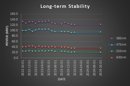
Long-term illumination stability
Long-term illumination stability measures the power output over the lifetime of the instrument. Over time, we expect a gradual decrease in power output due to the aging of hardware, including the light source and other optical components. These measurements are not an experiment per se but it is the measurement of the maximum power output over time.
Acquisition protocol
Results
Fill in the orange cells in the Illumination Stability_Template.xlsx spreadsheet to visualize your results. For each light source, plot the measured power output (in mW) over time to assess the stability of the illumination.
Calculate the relative power using the formula: Relative Power = Power / Max Power. Then, plot the Relative Power (%) over time.

Calculate the Relative PowerSpec by comparing the measured power to the manufacturer’s specifications using the following formula: Relative PowerSpec = Power / PowerSpec. Then, plot the Relative PowerSpec (% Spec) over time.

We expect a gradual decrease in power output over time due to the aging of hardware. Light sources should be replaced when the Relative PowerSpec falls below 50%.
Reports the results in a table.
| Stability Factor | Coefficient of Variation | |
| 385nm | 94.51% | 3.49% |
| 475nm | 93.59% | 4.42% |
| 555nm | 88.96% | 6.86% |
| 630nm | 89.46% | 6.71% |
Conclusion
Illumination stability conclusions
Real-time 1 min | Short-term 15 min | Mid-term 1 h | |
385nm | 99.99% | 100.00% | 99.98% |
475nm | 99.99% | 100.00% | 99.98% |
555nm | 99.97% | 100.00% | 99.99% |
630nm | 99.99% | 99.99% | 99.97% |
The light sources are highly stable (>99.9%).
Illumination Input-Output Linearity
This measure compares the power output as the input varies. A linear relationship is expected between the input and the power output.
Acquisition protocol
Results
Fill in the orange cells in the llumination Power Linearity_Template.xlsx spreadsheet to visualize your results. For each light source, plot the measured power output (in mW) as a function of the input (%).

Calculate the Relative Power using the formula: Relative Power = Power / MaxPower. Then, plot the Relative Power (%) as a function of the input (%).

Determine the equation for each curve, which is typically a linear relationship of the form: Output = K × Input. Report the slope (K) and the coefficient of determination (R²) for each curve in a table.
Illumination Input-Output Linearity | ||
Slope | R2 | |
385nm | 0.9969 | 1 |
475nm | 0.9984 | 1 |
555nm | 1.0012 | 1 |
630nm | 1.0034 | 1 |
The slopes demonstrate a nearly perfect linear relationship between the input and the measured output power, with values very close to 1. The coefficient of determination (R²) indicates a perfect linear fit, showing no deviation from the expected relationship.
Conclusion
Objectives and Cubes transmittance
Since we are using a power meter, we can easily assess the transmittance of the objectives and filter cubes. This measurement compares the power output when different objectives and filter cubes are in the light path. It evaluates the transmittance of each objective and compares it with the manufacturer’s specifications. This method can help detect defects or dirt on the objectives. It can also verify the correct identification of the filters installed in the microscope.
Objectives transmittance
Acquisition protocol
Results
Fill in the orange cells in the Objective and cube transmittance_Template.xlsx spreadsheet to visualize your results. For each objective, plot the measured power output (in mW) as a function of the wavelength (in nm).

Calculate the Relative Transmittance using the formula: Relative Transmittance = Power / PowerNoObjective. Then, plot the Relative Transmittance (%) as a function of the wavelength (in nm).

Calculate the average transmittance for each objective and report the results in a table. Compare the average transmittance to the specifications provided by the manufacturer to assess performance.
| Average Transmittance | Specifications [470-630] | Average Transmittance | |
| 2.5x-0.075 | 77% | >90% | 84% |
| 10x-0.25-Ph1 | 60% | >80% | 67% |
| 20x-0.5 Ph2 | 62% | >80% | 68% |
| 63x-1.4 | 29% | >80% | 35% |
The measurements are generally close to the specifications, with the exception of the 63x-1.4 objective. This deviation is expected, as the 63x objective has a smaller back aperture, which reduces the amount of light it can receive. Additionally, you can compare the shape of the transmittance curves to further assess performance.
Conclusion
Cubes transmittance
Acquisition protocol
Results
Fill in the orange cells in the Objective and cube transmittance_Template.xlsx spreadsheet to visualize your results. For each filter cube, plot the measured power output (in mW) as a function of the wavelength (in nm).

Calculate the Relative Transmittance using the formula: Relative Transmittance = Power / PowerMaxFilter. Then, plot the Relative Transmittance (%) as a function of the wavelength (in nm).

Calculate the average transmittance for each filter at the appropriate wavelengths and report the results in a table.
| 385 | 475 | 555 | 590 | 630 | |
| DAPI/GFP/Cy3/Cy5 | 100% | 100% | 100% | 100% | 100% |
| DAPI | 14% | 0% | 0% | 8% | 0% |
| GFP | 0% | 47% | 0% | 0% | 0% |
| DsRed | 0% | 0% | 47% | 0% | 0% |
| DHE | 0% | 0% | 0% | 0% | 0% |
| Cy5 | 0% | 0% | 0% | 0% | 84% |
The DAPI cube transmits only 14% of the excitation light compared to the Quad Band Pass DAPI/GFP/Cy3/Cy5. While it is still usable, it will provide a low signal. This is likely because the excitation filter within the cube does not match the light source properly. Since an excitation filter is already included in the light source, the filter in this cube could be removed.
The GFP and DsRed cubes transmit 47% of the excitation light compared to the Quad Band Pass DAPI/GFP/Cy3/Cy5, and they are functioning properly.
The DHE cube does not transmit any light from the Colibri. This cube may need to be removed and stored.
The Cy5 cube transmits 84% of the excitation light compared to the Quad Band Pass DAPI/GFP/Cy3/Cy5, and it is working properly.
Conclusion
We are done with the powermeter ![]() .
.
Field Illumination Uniformity
Now that we have confirmed the stability of our light sources and verified that the optical components (objectives and filter cubes) are transmitting light effectively, we can proceed to evaluate the uniformity of the illumination. This evaluates how uniform is the illumination
Acquisition protocol
Results
You should have acquired several multi-channel images that now need processing to yield meaningful results. To process them, use the Field Illumination analysis feature of the MetroloJ_QC plugin for FIJI.
- Open FIJI.
- Load your image by dragging it into the FIJI bar.
- Launch the MetroloJ_QC plugin by navigating to Plugins > MetroloJ QC.
- Click on Field Illumination Report.
- Enter a title for your report.
- Type in your name.
- Click Filter Parameters and input the filter's names, excitation, and emission wavelengths.
- Check Remove Noise using Gaussian Blur.
- Enable Apply Tolerance to the Report and reject uniformity and accuracy values below 80%.
- Click File Save Options.
- Select Save Results as PDF Reports
- Select Save Results as spreadsheets.
- Click OK.
- Repeat steps 4 through 13 for each image you have acquired.
This will generate detailed results, which will be stored in a folder named Processed. The Processed folder will be located in the same directory as the original images, with each report and result saved in its own subfolder.
Use the following R script to merge all _results.xls files into a single file.
This script will load all _results.xls files located in the "Input" folder on your desktop or prompt you to select an input folder.
It will compile and merge data generated by the MetroloJ_QC Field Illumination analysis, including metrics such as Uniformity and Centering Accuracy for each channel from every file.
Additionally, it will split the filenames using the _ character and create columns named Variable-001, Variable-002, etc. This will help in organizing the data if the filenames are formatted as Objective_VariableA_VariableB, for example.
The combined data will be saved as Combine_output.csv in the Output folder on your desktop.
# Clear the workspace
rm(list = ls())

# Set default input and output directories
default_input_dir <- file.path(Sys.getenv("USERPROFILE"), "Desktop", "Input")  # Default to "Input" on Desktop
InputFolder <- default_input_dir  # Use default folder

# Prompt user to select a folder (optional, currently commented)
InputFolder <- choose.dir(default = default_input_dir, caption = "Select an Input Folder") # You may comment this line if you want to directly use the InputFolder on your desktop

# If no folder is selected, fall back to the default
if (is.na(InputFolder)) {
  InputFolder <- default_input_dir
}

# Specify the Output folder (this is a fixed folder on the Desktop)
OutputFolder <- file.path(Sys.getenv("USERPROFILE"), "Desktop", "Output")
if (!dir.exists(OutputFolder)) dir.create(OutputFolder, recursive = TRUE)

# List all XLS files ending with "_results.xls" in the folder and its subfolders
xls_files <- list.files(path = InputFolder, pattern = "_results.xls$", full.names = TRUE, recursive = TRUE)
if (length(xls_files) == 0) stop("No _results.xls files found in the selected directory.")

# Define the header pattern to search for
header_pattern <- "Filters combination/set.*Uniformity.*Field Uniformity.*Centering Accuracy.*Image.*Coef. of Variation.*Mean c fit value"

# Initialize a list to store tables
all_tables <- list()

# Loop over all XLS files
for (file in xls_files) {
  # Read the file as raw lines (since it's tab-separated)
  lines <- readLines(file)

  # Find the line that matches the header pattern
  header_line_index <- grep(header_pattern, lines)

  if (length(header_line_index) == 0) {
    cat("No matching header found in file:", file, "\n")
    next  # Skip this file if the header isn't found
  }

  # Extract the table starting from the header row
  start_row <- header_line_index[1]

  # The table might end at an empty line, so let's find the next empty line after the header
  end_row <- min(grep("^\\s*$", lines[start_row:length(lines)]), na.rm = TRUE) + start_row - 1
  if (is.na(end_row)) end_row <- length(lines)  # If no empty line found, use the last line

  # Extract the table rows (lines between start_row and end_row)
  table_lines <- lines[start_row:end_row]

  # Convert the table lines into a data frame
  table_data <- read.table(text = table_lines, sep = "\t", header = TRUE, stringsAsFactors = FALSE)

  # Add the filename as the first column (without extension)
  filename_no_extension <- tools::file_path_sans_ext(basename(file))
  table_data$Filename <- filename_no_extension

  # Split the filename by underscores and add as new columns
  filename_parts <- unlist(strsplit(filename_no_extension, "_"))
  for (i in 1:length(filename_parts)) {
    table_data[[paste0("Variable-", sprintf("%03d", i))]] <- filename_parts[i]
  }

  # Rename columns based on the exact names found in the data
  colnames(table_data) <- gsub("Filters.combination.set", "Channel", colnames(table_data))
  colnames(table_data) <- gsub("Uniformity....", "Uniformity (%)", colnames(table_data))
  colnames(table_data) <- gsub("Field.Uniformity....", "Field Uniformity (%)", colnames(table_data))
  colnames(table_data) <- gsub("Centering.Accuracy....", "Centering Accuracy (%)", colnames(table_data))
  colnames(table_data) <- gsub("Coef..of.Variation", "CV", colnames(table_data))

  # Remove the "Mean.c.fit.value" column if present
  colnames(table_data) <- gsub("Mean.c.fit.value", "", colnames(table_data))

  # Drop any columns that were renamed to an empty string
  table_data <- table_data[, !grepl("^$", colnames(table_data))]

  # Divide the relevant columns by 100 to convert percentages into decimal values
  table_data$`Uniformity (%)` <- table_data$`Uniformity (%)` / 100
  table_data$`Field Uniformity (%)` <- table_data$`Field Uniformity (%)` / 100
  table_data$`Centering Accuracy (%)` <- table_data$`Centering Accuracy (%)` / 100

  # Store the table in the list with the file name as the name
  all_tables[[basename(file)]] <- table_data
}

# Check if any tables were extracted
if (length(all_tables) == 0) {
  stop("No tables were extracted from the files.")
}

# Optionally, combine all tables into a single data frame (if the structures are consistent)
combined_data <- do.call(rbind, all_tables)

# View the combined data
#head(combined_data)

# Optionally, save the combined data to a CSV file
output_file <- file.path(OutputFolder, "combined_output.csv")
write.csv(combined_data, output_file, row.names = FALSE)
cat("Combined data saved to:", output_file, "\n")
The following spreadsheet provides a dataset that can be manipulated with a pivot table to generate informative graphs and statistics Illumination_Uniformity_Template.xlsx. Plot the uniformity and centering accuracy for each objective.

| Objective | Uniformity | Centering Accuracy |
| 2x | 97.5% | 92.7% |
| 10x | 97.0% | 94.5% |
| 20x | 97.3% | 97.1% |
| 63x | 96.6% | 96.7% |
Plot the uniformity and centering accuracy for each filter set.

| Filter | Uniformity | Centering Accuracy |
| DAPI | 98.3% | 99.4% |
| DAPIc | 95.8% | 84.9% |
| GFP | 98.1% | 99.1% |
| GFPc | 96.5% | 93.3% |
| Cy3 | 97.6% | 96.5% |
| Cy3c | 96.8% | 97.9% |
| Cy5 | 97.0% | 99.6% |
| Cy5c | 96.7% | 91.3% |
This specific instrument has a quad-band filter as well as individual filter cubes. We can plot the uniformity and centering accuracy per filter types.

| Filter Type | Uniformity | Centering Accuracy |
Quad band | 97.7% | 98.7% |
| Single band | 96.5% | 91.8% |
Finally store the original field illumination images to be able to perform shading corrections.
Conclusion
XYZ Drift
This experiment assesses the stability of the system in the XY and Z directions. As previously noted, when an instrument is started, it requires time to reach a stable steady state, a phase known as the warmup period. To accurately determine this duration, it is essential to record a warmup kinetic at least once a year.
Acquisition protocol
Results
- Use the TrackMate plugin for FIJI to detect and track spots over time
- Apply Difference of Gaussians (DoG) spot detection with a detection size of 4 µm
- Set a quality threshold greater than 20 and enable sub-pixel localization for increased accuracy
- Export the detected spot coordinates as a CSV file for further analysis
Fill in the orange cells in the following spreadsheet template XYZ Drift Kinetic_Template.xlsx. to visualize your results. Just copy paste XYZT and Frame columns from trackmate spots CSV file to the orange column in the XLSX file. Fill in the NA and Emission wavelength used.
Calculate the relative displacement in X, Y and Z: Relative Displacement = Position - PositionInitial and plot the relative displacement over time.

We observe an initial drift that stabilizes over time in X (+2 um), Y (+1.3 um) and Z (-10.5 um).
Calculate the displacement 3D Displacement = Sqrt( (X2-X1)2 + (Y2-Y1)2) + (Z2-Z1)2 ) and plot the displacement over time. Calculate the resolution of your imaging configuration, Lateral Resolution = LambdaEmission / 2*NA and plot the resolution over time (constant).

Identify visually the time when the displacement is lower than the resolution of the system. On this instrument it takes 120 min to reach its stability.
Calculate the velocity, Velocity = (Displacement2-Displacement1)/T2-T1) and plot the velocity over time.

Calculate the average velocity before and after stabilisation and report the results in a table
| Objective NA | 0.5 |
| Wavelength (nm) | 705 |
| Resolution (nm) | 705 |
| Stabilisation time (min) | 122 |
| Average velocity Warmup (nm/min) | 113 |
| Average velocity System Ready (nm/min) | 14 |
Conclusion
XYZ Repositioning accuracy
This experiment evaluates how accurate is the system in XY by measuring the accuracy of repositioning. Several variables can affect repositioning accuracy: i) Time, ii) Traveled distance, iii) Speed and iv) acceleration.
Acquisition protocol
- Place 4 um diameter fluorescent beads (TetraSpec Fluorescent Microspheres Size Kit mounted on slide) on the stage.
- Center the sample under a high NA dry objective.
- Select an imaging channel (e.g., Cy5)
Acquire a Z-stack at 2 different positions separated by 0 um, 1 um, 10 um, 100 um, 1 000 um, 10 000 um, 80 000um in X and Y direction
Repeat the acquisition 20 times
Be careful your stage might have a smaller range!
Be careful not to damage the objectives (lower the objectives during movement)
I recommend to acquire 3 dataset for each condition.
Results
- Use the TrackMate plugin for FIJI to detect and track spots over time
- Apply Difference of Gaussians (DoG) spot detection with a detection size of 1 µm
- Set a quality threshold greater than 20 and enable sub-pixel localization for increased accuracy
- Export the detected spot coordinates as a CSV file for further analysis
Fill in the orange cells in the following spreadsheet template XY Repositioning Accuracy_Template.xlsx. to visualize your results. Just copy paste XYZT and Frame columns from trackmate spots CSV file to the orange column in the XLSX file. Fill in the NA and Emission wavelength used.


This experiment shows the displacement in X, Y and Z after + and - 30mm movement in X and Y, repeated 20 times.
Report the results in a table.
| Objective NA | 0.5 |
| Wavelength (nm) | 705 |
| Lateral Resolution (nm) | 705 |
| X Accuracy (nm) | 195 |
| Y Accuracy (nm) | 175 |
| Z Accuracy (nm) | 52 |
| Repositioning Accuracy 3D (nm) | 169 |
| Repositioning Accuracy 2D (nm) | 178 |
Because several variables can affect repositioning accuracy (i) Time, ii) Traveled distance, iii) Speed and iv) Acceleration) we decided to test them. To do this we use the following code to automatically process an opened image in ImageJ/FIJI using the Trackmate plugin. It will save the spot detection as a CSV file on your Desktop.
This should create a lot of CSV Files that we need to be aggregated for the following analysis. The following script in R can process all csv files placed in an Output folder on your desktop.
This script calculates the relative position in X, Y and Z: PositionRelative= Position - PositionInitialfor each axes eind each file. It also calculates the 2D and 3D displacement: 2D_Displacement = Sqrt( (X2-X1)2 + (Y2-Y1)2)); 3D_Displacement = Sqrt( (X2-X1)2 + (Y2-Y1)2) + (Z2-Z1)2 ) and provides the results as CSV file merged_data.csv that can be further processed and summarized with a pivot table XY Repositioning Accuracy_Template_All-Files.xlsx
Repositioning accuracy vs Traveled Distance
Plot the 3D displacement for each condition function of the acquisition frame.

We observe here a high variability at the Frame 1 (2nd image). This variability can comes from the X, Y or Z axis. I can also come from a combination of those 3. We now plot the displacement in each direction function of the Frame.


We observe that the X axis is contributing to the high variability of the first frame. Ploting the 3D displacement as a scatter dotplot for each condition and repeat.

We observe that the recorded data is consistent at the exception of a single value per condition.


In these graphs we observe the variability per experiment. Notice that most of the experiment show a shift in X and some in Y. Data is then more consistent.

Travelled distance significantly affect the repositioning accuracy at 1mm, 10mm and 30mm.


Repositioning accuracy vs Speed and Acceleration
