
This page provides a practical guide for microscope quality control. By following the outlined steps, utilizing the provided template files, and running the included scripts, you will have everything needed to easily generate comprehensive report on your microscope's performance.
Equipment used
- Thorlabs Power Meter (PM400) and sensor (S170C)
- Thorlabs Fluorescent Slides (FSK5)
- TetraSpeck™ Fluorescent Microspheres Size Kit (mounted on slide) ThermoFisher (T14792)
Software used
- FIJI FIJI
- MetroloJ_QC Plugin for FIJI MetroloJ_QC
- iText Plugin for FIJI iText
- R R from the CRAN R Project
- I typically use RStudio the integrated development environment (IDE) for R
Please note that during quality control, you may, and likely will, encounter defects or unexpected behavior. This practical guide is not intended to assist with investigating or resolving these issues. With that said, we wish you the best of luck and are committed to providing support. Feel free to reach out to us at microscopie@cib.umontreal.ca
Illumination Warmup Kinetic
When starting light sources, they require time to reach a stable and steady state. This duration is referred to as the warm-up period. To ensure accurate performance, it is essential to record the warm-up kinetics at least once a year to precisely define this period. For a detailed exploration of illumination stability, refer to the Illumination Power, Stability, and Linearity Protocol by the QuaRep Working Group 01.
Acquisition protocol
Results
Use the provided spreadsheet template, Illumination_Warmup Kinetic_Template.xlsx, and fill in the orange cells to visualize your results. For each light source, plot the measured power output (in mW) against time to analyze the data.

Calculate the relative power using the formula: Relative Power = (Power / Max Power). Then, plot the Relative Power (%) against time to visualize the data.

We observe some variability in the power output for the 385 nm light source.
To assess the stability:
Define a Stability Duration Window:
Select a time period (e.g., 10 minutes) during which the power output should remain stable.Specify a Maximum Coefficient of Variation (CV) Threshold:
Determine an acceptable variability limit for the selected window (e.g., 0.01%).Calculate the Coefficient of Variation (CV):
Use the formula: CV = (Standard Deviation / Mean)
Compute the CV for the specified stability duration window.Visualize Stability:
Plot the calculated CV over time to analyze the stability of the power output.


We observe that the light sources stabilize quickly, within less than 10 minutes, while the 385 nm light source takes approximately 41 minutes to reach the stability threshold. The template also calculates Stability Factor (S) using the formula: S (%) = 100 × (1 - (Pmax - Pmin) / (Pmax + Pmin))
Report the results in a table
| 385nm | 475nm | 555nm | 630nm | |
| Stabilisation time (Max CV 0.01% for 10 min) | 41 | 3 | 3 | 8 |
| Stability Factor (%) Before Warmup | 99.7% | 99.9% | 100.0% | 100.0% |
| Stability Factor (%) After Warmup | 100.0% | 100.0% | 100.0% | 99.9% |
Selected Stability Duration Window (min): 10 min and Maximum Coefficient of Variation: 0.01%.
Metrics
- The Stability Factor indicates a higher stability the closer to 100% and focuses specifically on the range of values (difference between max and min) relative to their sum, providing an intuitive measure of how tightly the system's behavior stays within a defined range.
- The Coefficient of Variation focuses on the dispersion of all data points (via the standard deviation) relative to the mean. Lower Coefficient indicates a better stability around the mean.
Conclusion
Illumination Maximum Power Output
This measure assesses the maximum power output of each light source, considering both the quality of the light source and the components along the light path. Over time, we expect a gradual decrease in power output due to the aging of hardware, including the light source and other optical components. These measurements will also be used to track the performance of the light sources over their lifetime (see Long-Term Illumination Stability section). For a detailed exploration of illumination properties, refer to the Illumination Power, Stability, and Linearity Protocol by the QuaRep Working Group 01.
Acquisition protocol
Results
Fill in the orange cells in the Illumination_Maximum Power Output_Template.xlsx spreadsheet to visualize your results. For each light source, plot the measured maximum power output (in mW).

Plot the measured maximum power output (in mW) and compare it to the manufacturer’s specifications. Calculate the Relative Power using the formula: Relative Power = (Measured Power / Manufacturer Specifications) and plot the relative power for each light source

Report the results in a table
| Manufacturer Specifications (mW) | Measurements 2024-11-22 (mW) | Relative Power (%) | |
| 385nm | 150.25 | 122.2 | 81% |
| 470nm | 110.4 | 95.9 | 87% |
| 555nm | 31.9 | 24 | 75% |
| 630nm | 52 | 39.26 | 76% |
Metrics
- The Maximum Power indicates how much light is provided by the instrument.
- The Relative Power to Specificaitons indicates how much power is provided compared to the specifications.
Conclusion
Illumination Stability
The light sources used on a microscope should remain constant or at least stable over the time scale of an experiment. For this reason, illumination stability is recorded across four different time scales:
- Real-time Illumination Stability: Continuous recording for 1 minute. This represents the duration of a z-stack acquisition.
- Short-term Illumination Stability: Recording every 1-10 seconds for 5-15 minutes. This represents the duration needed to acquire several images.
- Mid-term Illumination Stability: Recording every 10-30 seconds for 1-2 hours. This represents the duration of a typical acquisition session or short time-lapse experiments. For longer time-lapse experiments, a longer duration may be used.
- Long-term Illumination Stability: Recording once a year or more over the lifetime of the instrument.
For a detailed exploration of illumination stability, refer to the Illumination Power, Stability, and Linearity Protocol by the QuaRep Working Group 01.
Real-time Illumination Stability
Acquisition protocol
Results
Fill in the orange cells in the Illumination_Stability_Template.xlsx spreadsheet to visualize your results. For each light source, plot the measured power output (in mW) over time.

Calculate the relative power using the formula: Relative Power = (Power / Max Power). Then, plot the Relative Power (%) over time.

Calculate the Stability Factor (S) using the formula: S (%) = 100 × (1 - (Pmax - Pmin) / (Pmax + Pmin)). Also, calculate the Coefficient of Variation (CV) using the formula: CV = Standard Deviation / Mean.
Reports the results in a table.
| Stability Factor | Coefficient of Variation | |
| 385nm | 99.99% | 0.002% |
| 475nm | 99.99% | 0.002% |
| 555nm | 99.97% | 0.004% |
| 630nm | 99.99% | 0.002% |
From the Stability Factor results, we observe that the difference between the maximum and minimum power is less than 0.03%. Additionally, the Coefficient of Variation indicates that the standard deviation is less than 0.004% of the mean value, demonstrating excellent power stability.
Conclusion
Short-term Illumination Stability
Acquisition protocol
Results
Fill in the orange cells in the Illumination_Stability_Template.xlsx spreadsheet to visualize your results. For each light source, plot the measured power output (in mW) over time.

Calculate the relative power using the formula: Relative Power = Power / Max Power. Then, plot the Relative Power (%) over time.

Calculate the Stability Factor (S) using the formula: S (%) = 100 × (1 - (Pmax - Pmin) / (Pmax + Pmin)). Also, calculate the Coefficient of Variation (CV) using the formula: CV = Standard Deviation / Mean.
Reports the results in a table.
| Stability Factor | Coefficient of Variation | |
| 385nm | 100.00% | 0.000% |
| 475nm | 100.00% | 0.002% |
| 555nm | 100.00% | 0.003% |
| 630nm | 99.99% | 0.004% |
From the Stability Factor results, we observe that the difference between the maximum and minimum power is less than 0.01%. Additionally, the Coefficient of Variation indicates that the standard deviation is less than 0.004% of the mean value, demonstrating excellent power stability.
Conclusion
Mid-term Illumination Stability
Acquisition protocol
Results
Fill in the orange cells in the Illumination_Stability_Template.xlsx spreadsheet to visualize your results. For each light source, plot the measured power output (in mW) over time to assess stability.

Calculate the relative power using the formula: Relative Power = Power / Max Power. Then, plot the Relative Power (%) over time.

Calculate the Stability Factor (S) using the formula: S (%) = 100 × (1 - (Pmax - Pmin) / (Pmax + Pmin)). Also, calculate the Coefficient of Variation (CV) using the formula: CV = Standard Deviation / Mean. Reports the results in a table.
| Stability Factor | Coefficient of Variation | |
| 385nm | 99.98% | 0.013% |
| 475nm | 99.98% | 0.011% |
| 555nm | 99.99% | 0.007% |
| 630nm | 99.97% | 0.020% |
From the Stability Factor results, we observe that the difference between the maximum and minimum power is less than 0.03%. Additionally, the Coefficient of Variation indicates that the standard deviation is less than 0.02% of the mean value, demonstrating excellent power stability.
Conclusion
Long-term Illumination Stability
Long-term illumination stability measures the power output over the lifetime of the instrument. Over time, we expect a gradual decrease in power output due to the aging of hardware, including the light source and other optical components. These measurements are not an experiment per se but it is the measurement of the maximum power output over time.
Acquisition protocol
Results
Fill in the orange cells in the Illumination_Stability_Template.xlsx spreadsheet to visualize your results. For each light source, plot the measured power output (in mW) over time to assess the stability of the illumination.
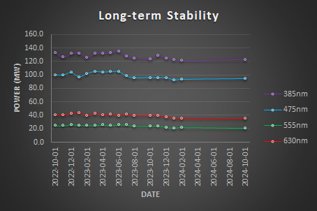
Calculate the relative power using the formula: Relative Power = Power / Max Power. Then, plot the Relative Power (%) over time.

Calculate the Relative PowerSpec by comparing the measured power to the manufacturer’s specifications using the following formula: Relative PowerSpec = Power / PowerSpec. Then, plot the Relative PowerSpec (% Spec) over time.

We expect a gradual decrease in power output over time due to the aging of hardware. Light sources should be replaced when the Relative PowerSpec falls below 50%.
Reports the results in a table.
| Stability Factor | Coefficient of Variation | |
| 385nm | 94.51% | 3.49% |
| 475nm | 93.59% | 4.42% |
| 555nm | 88.96% | 6.86% |
| 630nm | 89.46% | 6.71% |
Conclusion
Illumination Stability Conclusions
| Stability Factor | Real-time 1 min | Short-term 15 min | Mid-term 1 h |
385nm | 99.99% | 100.00% | 99.98% |
475nm | 99.99% | 100.00% | 99.98% |
555nm | 99.97% | 100.00% | 99.99% |
630nm | 99.99% | 99.99% | 99.97% |
The light sources are highly stable (Stability >99.9%).
Metrics
- The Stability Factor indicates a higher stability the closer to 100% and focuses specifically on the range of values (difference between max and min) relative to their sum, providing an intuitive measure of how tightly the system's behavior stays within a defined range.
- The Coefficient of Variation focuses on the dispersion of all data points (via the standard deviation) relative to the mean. Lower Coefficient indicates a better stability around the mean.
Illumination Input-Output Linearity
This measure compares the power output as the input varies. A linear relationship is expected between the input and the power output. For a detailed exploration of illumination linearity, refer to the Illumination Power, Stability, and Linearity Protocol by the QuaRep Working Group 01.
Acquisition protocol
Results
Fill in the orange cells in the Illumination_Linearity_Template.xlsx spreadsheet to visualize your results. For each light source, plot the measured power output (in mW) as a function of the input (%).

Calculate the Relative Power using the formula: Relative Power = Power / MaxPower. Then, plot the Relative Power (%) as a function of the input (%).

Determine the equation for each curve, which is typically a linear relationship of the form: Output = K × Input. Report the slope (K) and the coefficient of determination (R²) for each curve in a table.
Illumination Input-Output Linearity | ||
Slope | R2 | |
385nm | 0.9969 | 1 |
475nm | 0.9984 | 1 |
555nm | 1.0012 | 1 |
630nm | 1.0034 | 1 |
The slopes demonstrate a nearly perfect linear relationship between the input and the measured output power, with values very close to 1. The coefficient of determination (R²) indicates a perfect linear fit, showing no deviation from the expected relationship.
Metrics
- The Slope indicates the rate of change between Input and Ouput.
- The Coefficient of Determination indicates how fitted is the data to a linear relationship.
Conclusion
Objectives and Cubes Transmittance
Since we are using a power meter, we can easily assess the transmittance of the objectives and filter cubes. This measurement compares the power output when different objectives and filter cubes are in the light path. It evaluates the transmittance of each objective and compares it with the manufacturer’s specifications. This method can help detect defects or dirt on the objectives. It can also verify the correct identification of the filters installed in the microscope.
Objectives Transmittance
Acquisition protocol
Results
Fill in the orange cells in the Objective and cube transmittance_Template.xlsx spreadsheet to visualize your results. For each objective, plot the measured power output (in mW) as a function of the wavelength (in nm).

Calculate the Relative Transmittance using the formula: Relative Transmittance = Power / PowerNoObjective. Then, plot the Relative Transmittance (%) as a function of the wavelength (in nm).

Calculate the average transmittance for each objective and report the results in a table. Compare the average transmittance to the specifications provided by the manufacturer to assess performance.
| Average Transmittance | Specifications [470-630] | Average Transmittance | |
| 2.5x-0.075 | 77% | >90% | 84% |
| 10x-0.25-Ph1 | 60% | >80% | 67% |
| 20x-0.5 Ph2 | 62% | >80% | 68% |
| 63x-1.4 | 29% | >80% | 35% |
The measurements are generally close to the specifications, with the exception of the 63x-1.4 objective. This deviation is expected, as the 63x objective has a smaller back aperture, which reduces the amount of light it can receive. Additionally, you can compare the shape of the transmittance curves to further assess performance.
Conclusion
Cubes Transmittance
Acquisition protocol
Results
Fill in the orange cells in the Objective and cube transmittance_Template.xlsx spreadsheet to visualize your results. For each filter cube, plot the measured power output (in mW) as a function of the wavelength (in nm).

Calculate the Relative Transmittance using the formula: Relative Transmittance = Power / PowerMaxFilter. Then, plot the Relative Transmittance (%) as a function of the wavelength (in nm).

Calculate the average transmittance for each filter at the appropriate wavelengths and report the results in a table.
| 385 | 475 | 555 | 590 | 630 | |
| DAPI/GFP/Cy3/Cy5 | 100% | 100% | 100% | 100% | 100% |
| DAPI | 14% | 0% | 0% | 8% | 0% |
| GFP | 0% | 47% | 0% | 0% | 0% |
| DsRed | 0% | 0% | 47% | 0% | 0% |
| DHE | 0% | 0% | 0% | 0% | 0% |
| Cy5 | 0% | 0% | 0% | 0% | 84% |
The DAPI cube transmits only 14% of the excitation light compared to the Quad Band Pass DAPI/GFP/Cy3/Cy5. While it is still usable, it will provide a low signal. This is likely because the excitation filter within the cube does not match the light source properly. Since an excitation filter is already included in the light source, the filter in this cube could be removed.
The GFP and DsRed cubes transmit 47% of the excitation light compared to the Quad Band Pass DAPI/GFP/Cy3/Cy5, and they are functioning properly.
The DHE cube does not transmit any light from the Colibri. This cube may need to be removed and stored.
The Cy5 cube transmits 84% of the excitation light compared to the Quad Band Pass DAPI/GFP/Cy3/Cy5, and it is working properly.
Conclusion
We are done with the powermeter ![]() .
.
Field Illumination Uniformity
Having confirmed the stability of our light sources and verified that the optical components (objectives and filter cubes) are transmitting light effectively, we can now proceed to evaluate the uniformity of the illumination. This step assesses how evenly the illumination is distributed. For a comprehensive guide on illumination uniformity, refer to the Illumination Uniformity by the QuaRep Working Group 03.
Acquisition protocol
Processing
Results
Plot the uniformity and centering accuracy for each objective.
Metrics
- The Uniformity indicates the range between the minimum and maximum intensities in the image. U=(Min/Max)*100. 100% Uniformity indicates a perfectly homogeneous image. 50% Uniformity indicates the minimum is half the maximum.
- The Centering Accuracy indicates how far from the center of the image is the center of the illumination (centroid of the max illumination bin). 100% indicates a perfectly aligns with the center of the image. 0% centering accuracy indicates that the center of the illumination is the farthest from the center of the image.

| Objective | Uniformity | Centering Accuracy |
| 2x | 97.5% | 92.7% |
| 10x | 97.0% | 94.5% |
| 20x | 97.3% | 97.1% |
| 63x | 96.6% | 96.7% |
Plot the uniformity and centering accuracy for each filter set.

| Filter | Uniformity | Centering Accuracy |
| DAPI | 98.3% | 99.4% |
| DAPIc | 95.8% | 84.9% |
| GFP | 98.1% | 99.1% |
| GFPc | 96.5% | 93.3% |
| Cy3 | 97.6% | 96.5% |
| Cy3c | 96.8% | 97.9% |
| Cy5 | 97.0% | 99.6% |
| Cy5c | 96.7% | 91.3% |
This specific instrument has a quad-band filter as well as individual filter cubes. We can plot the uniformity and centering accuracy per filter types.

| Filter Type | Uniformity | Centering Accuracy |
Quad band | 97.7% | 98.7% |
| Single band | 96.5% | 91.8% |
Conclusion
XYZ Drift
This experiment evaluates the stability of the system in the XY and Z directions. As noted earlier, when an instrument is started, it requires a warmup period to reach a stable steady state. To determine the duration of this phase accurately, it is recommended to record a warmup kinetic at least once per year. For a comprehensive guide on Drift and Repositioning, refer to the Stage and Focus Precision by the QuaRep Working Group 06.
Acquisition protocol
Processing
Results
- Open the spreadsheet template XYZ Drift Kinetic_Template.xlsx and fill in the orange cells.
- Copy and paste the XYZT and Frame columns from the TrackMate spots CSV file into the corresponding orange columns in the spreadsheet.
- Enter the numerical aperture (NA) and emission wavelength used during the experiment.
- Calculate the relative displacement in X, Y, and Z using the formula: Relative Displacement = Position - PositionInitial.
- Finally, plot the relative displacement over time to visualize the system's drift.


Identify visually the time when the displacement is lower than the resolution of the system. On this instrument it takes 120 min to reach its stability. Calculate the velocity, Velocity = (Displacement2-Displacement1)/T2-T1) and plot the velocity over time.

Calculate the average velocity before and after stabilisation and report the results in a table.
| Objective NA | 0.5 |
| Wavelength (nm) | 705 |
| Resolution (nm) | 705 |
| Stabilisation time (min) | 122 |
| Average velocity Warmup (nm/min) | 113 |
| Average velocity System Ready (nm/min) | 14 |
Metrics
- The Stabilisation Time indicates the time in minutes necessary for the instrument to have a drift lower than the resolution of the system.
- The Average Velocity indicates the speed of drift in all directions XYZ in nm/min.
Conclusion
Stage Repositioning Dispersion
This experiment evaluates how accurate is the system in XY by measuring the dispersionof repositioning. Several variables can affect repositioning: i) Time, ii) Traveled distance, iii) Speed and iv) acceleration. For a comprehensive guide on Stage Repositioning, refer to the Stage and Focus Precision by the QuaRep Working Group 06 and the associated XY Repositioning Protocol.
Acquisition protocol
Processing
Results
- Open the spreadsheet template Stage Repositioning Dispersion_Template.xlsx and fill in the orange cells.
- Copy and paste the XYZT and Frame columns from the TrackMate spots CSV file into the corresponding orange columns in the spreadsheet.
- Enter the numerical aperture (NA) and emission wavelength used during the experiment.
- Calculate the relative position in X, Y, and Z using the formula: Relative PositionRelative = Position - PositionInitial.
- Finally, plot the relative position over time to visualize the system's stage repositioning dispersion.


We observe an initial movement in X and Y that stabilises. Calculate the displacement 2D Displacement = Sqrt( (X2-X1)2 + (Y2-Y1)2) ) and plot the 2D displacement over time. Calculate the resolution of your imaging configuration, Lateral Resolution = LambdaEmission / 2*NA and plot the resolution over time (constant).

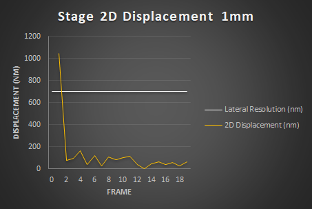

This experiment shows a significant initial displacement between Frame 0 and Frame 1, ranging from 1000 nm to 400 nm, which decreases to 70 nm by Frame 2. To quantify this variation, calculate the dispersion for each displacement using the formula: Dispersion = StandardDeviation(Displacement). Report the results in a table.
| Traveled Distance (mm) | 0 mm | 1 mm | 10 mm |
| X Dispersion (nm) | 4 | 188 | 121 |
| Y Dispersion (nm) | 4 | 141 | 48 |
| Z Dispersion (nm) | 10 | 34 | 53 |
| Repositioning Dispersion 3D (nm) | 6 | 227 | 91 |
| Repositioning Dispersion 2D (nm) | 2 | 226 | 90 |
Conclusion
Further Investigation
We observed a significant shift in the first frame, which was unexpected and invites further investigation. These variables can affect repositioning dispersion: i) Traveled distance, ii) Speed, iii) Acceleration, iv) Time, and v) Environment. We decided to test the first three.
Methodology
Processing
This experimental protocol generated a substantial number of images. To process them automatically in ImageJ/FIJI using the TrackMate plugin, we use the following script Stage Repositioning with Batch TrackMate-v5.py
This script automates the process of detecting and tracking spots using the TrackMate plugin for ImageJ/FIJI. To use it:
- Drop the script into the FIJI toolbar and click Run.
This script generates a CSV file for each image, which can be aggregated for further analysis using the accompanying R script, Process Stage Repositioning Results.R. This R script processes all CSV files in a selected folder and save the file as XYZ_Repositioning_Merged-Data.csv in an "Output" folder on the user desktop for streamlined data analysis.
This R code automates the processing of multiple CSV files containing spot tracking data.
This script generate a single CSV File that can be further processed and summarized with a pivot table as shown in the following spreadsheet Stage-Repositioning_Template.xlsx
Using the first frame as a reference we can plot the average XYZ position for each frame.

As observed earlier, there is a significant displacement between Frame 0 and Frame 1, particularly along the X-axis. For this analysis, we will exclude the first two frames and focus on the variables of interest: (i) Traveled distance, (ii) Speed, and (iii) Acceleration and will come back to the initial shift later.
Repositioning Dispersion: Impact of Traveled Distance
Results
Plot the 2D displacement versus the frame number for each condition of traveled distance.

The data looks good now with the two first frames ignored. Now, we can calculate the average of the standard deviation of the 2D displacement and plot these values against the traveled distance..

We observe a power-law relationship, described by the equation: Repositioning Dispersion = 8.2 x Traveled Distance^0.2473
| Traveled Distance (um) | Repositioning Dispersion (nm) |
| 0 | 4 |
| 1 | 6 |
| 10 | 20 |
| 100 | 19 |
| 1000 | 76 |
| 10000 | 56 |
| 30000 | 107 |

Conclusion
Repositioning Dispersion: Impact of Speed and Acceleration
Results
Generate a plot of the 2D displacement as a function of frame number for each combination of Speed and Acceleration conditions. This visualization will help assess the relationship between displacement and time across the different experimental settings.

As noted earlier, there is a significant displacement between Frame 0 and Frame 1, particularly along the X-axis (600 nm) and, to a lesser extent, the Y-axis (280 nm). To refine our analysis, we will exclude the first two frames and focus on the key variables of interest: (i) Speed and (ii) Acceleration. To better understand the system's behavior, we will visualize the average standard deviation of the 2D displacement for each combination of Speed and Acceleration conditions.


Our observations indicate that both Acceleration and Speed contribute to an increase in 2D repositioning dispersion. However, a two-way ANOVA reveals that only Speed has a statistically significant effect on 2D repositioning dispersion. Post-hoc analysis further demonstrates that the dispersion for the Speed-Fast, Acc-High condition is significantly greater than that of the Speed-Low, Acc-Low condition.
| 2D Repositioning Dispersion (nm) | |
| Speed-Slow Acc-Low | 32 |
| Speed-Slow Acc-High | 49 |
| Speed-Fast Acc-Low | 54 |
| Speed-Fast Acc-High | 78 |
Conclusion
What about the initial shift ?
Right, I almost forgot about that. See below.
Results
Ploting the 3D displacement for each tested conditions from the preivous data.


We observe a single floating point that corresponds to the displacement between Frame 0 and Frame 1. This leads me to hypothesize that the discrepancy may be related to the stage's dual motors, each controlling a separate axis (X and Y). Each motor operates in two directions (Positive and Negative). Since the shift occurs only at the first frame, this likely relates to how the experiment is initiated.
To explore this further, I decided to test whether these variables significantly impact the repositioning. We followed the XYZ repositioning dispersion protocol, testing the following parameters:
- Distance: 1000 µm
- Speed: 100%
- Acceleration: 100%
- Axis: X, Y, XY
- Starting Point: Centered (on target), Positive (shifted positively from the reference position), Negative (shifted negatively from the reference position)
- For each condition, three datasets were acquired.
Data Stage-Repositining_Diagnostic-Data.xlsx was processed as mentioned before and we ploted the 2D displacement function of the frame for each condition.

When moving along the X-axis only, we observe a shift in displacement when the starting position is either centered or positively shifted, but no shift occurs when the starting position is negatively shifted. This suggests that the behavior of the stage’s motor or the initialization of the experiment may be affected by the direction of the shift relative to the reference position, specifically when moving in the positive direction.

When moving along the Y-axis only, we observe a shift in displacement when the starting position is positively shifted, but no shift occurs when the starting position is either centered or negatively shifted. This indicates that the stage's motor behavior or initialization may be influenced by the direction of the shift, particularly when starting from a positive offset relative to the reference position.

When moving along both the X and Y axes simultaneously, a shift is observed when the starting position is centered. This shift becomes more pronounced when the starting position is positively shifted in any combination of the X and Y axes (+X+Y, +X-Y, -X+Y). However, the shift is reduced when the starting position is negatively shifted along both axes.
Conclusion
Channel Co-Alignment
Channel co-alignment or co-registration refers to the process of aligning image data collected from multiple channels. This ensures that signals originating from the same location in the sample are correctly overlaid. This process is essential in multi-channel imaging to maintain spatial accuracy and avoid misinterpretation of co-localized signals. For a comprehensive guide on Channel Co-Registration, refer to the Chromatic aberration and Co-Registration the QuaRep Working Group 04.
Acquisition protocol
Processing
Results
The following spreadsheet provides a dataset that can be manipulated with a pivot table to generate informative graphs and statistics Channel_Co-registration_Template.xlsx.
Metrics
- The Nyquist ratio evaluates how closely the images align with the Nyquist sampling criterion. It is calculated as: Nyquist Ratio = Pixel Dimension / Nyquist Dimension
- A ratio of 1 indicates that the image acquisition complies with the Nyquist criterion.
- A ratio above 1 signifies that the pixel dimensions of the image exceed the Nyquist criterion.
- A ratio below 1 is the desired outcome, as it ensures proper sampling.
- The Co-Registration Ratios measure the spatial alignment between two channels by comparing the distance between the centers of corresponding beads in both channels to a reference distance. The reference distance is defined as the size of the fitted ellipse around the bead in the first channel.
- A ratio of 1 means the center of the bead in the second channel is located on the edge of the ellipse fitted around the bead in the first channel.
- A ratio above 1 indicates the center of the bead in the second channel lies outside the ellipse around the first channel's bead center.
- A ratio below 1 is the desired outcome, indicating that the center of the bead in the second channel is within a range smaller than the system's 3D resolution.
This method is the approach used in the MetroloJ QC Channel Co-Registration function. In my personal opinion n ellipse with a height equal to the Z-resolution and a width equal to the XY-resolution would intuitively be OK for this analysis.
Because the data is complex we will start with an overal look at the data before progressively diving into more complex analysis. Plot the average co-registration ratio for each objective.

The average co-registration ratio are below 1.0 for all objectives excepted for the 10x. Plot the average co-registration ratios for each Channel (Regarless of the objective used and of the channel pairing).

The average co-registration ratio are above 1.0 for the DAPI, equal to 1.0 for GFP and below 1 for the Cy3 and Cy5 Channels. Plot the average Co-Registration ratios for each Channel and each objective (regarless of the channel pairing).

The average co-registration ratio are above 1.0 for the DAPI 2x, 10x and 20x, GFP 2x and 10x. Plot the average Co-Registration ratios for every combination of 2 channels (regarless of the objective used).

The DAPI channel has an average co-registration ratio above 1 for the matching with Cy3 and Cy5 channels but not with GFP. The GFP channel aboev 1 for the pairing with Cy5. The Cy3 channel has an average co-registration ratio above 1 for the pariing with DAPI. The Cy5 channel has an average co-registration ratio above 1 for the pairing with DAPI and GFP channels. A co-registration ratio above 1 indicates that the distance of the localisation of the center of the bead in the two channels is higher than the resolution of the system (longest wavelength is used for the calculation of the resolution).
The table below indicates the ratio for each objective and each pair of channels.

Why should you care? Well when you are acquiring a multi-channel image you might see a significant shift between the two channels. This is particularly true for the combination of DAPI and Cy3 channels with the 10x Objective.


Report the Pixel Shift Table For each objective and each filter combination. This table can (should) be used to correct a multi-channel image by displacing the Channel 2 relative to the Channel 1 by the XYZ pixel coordinates indicated.
| Channel_2 | ||||||
| Objective | Channel_1 | Axis | DAPI | GFP | Cy3 | Cy5 |
| 2x | DAPI | X | 0.89 | -0.14 | -0.35 | |
| Y | 0.19 | 1.63 | 2.00 | |||
| Z | 0.89 | 3.67 | 1.58 | |||
| GFP | X | -0.89 | -1.04 | -1.25 | ||
| Y | -0.19 | 1.44 | 1.81 | |||
| Z | -0.89 | 2.78 | 0.70 | |||
| Cy3 | X | 0.14 | 1.04 | -0.21 | ||
| Y | -1.63 | -1.44 | 0.37 | |||
| Z | -3.67 | -2.78 | -2.08 | |||
| Cy5 | X | 0.35 | 1.25 | 0.21 | ||
| Y | -2.00 | -1.81 | -0.37 | |||
| Z | -1.58 | -0.70 | 2.08 | |||
| 10x | DAPI | X | 0.46 | -0.85 | -1.16 | |
| Y | 0.50 | 1.79 | 2.27 | |||
| Z | 4.22 | 4.44 | 1.91 | |||
| GFP | X | -0.46 | -1.31 | -1.61 | ||
| Y | -0.50 | 1.29 | 1.77 | |||
| Z | -4.22 | 0.22 | -2.31 | |||
| Cy3 | X | 0.85 | 1.31 | -0.30 | ||
| Y | -1.79 | -1.29 | 0.48 | |||
| Z | -4.44 | -0.22 | -2.53 | |||
| Cy5 | X | 1.16 | 1.61 | 0.30 | ||
| Y | -2.27 | -1.77 | -0.48 | |||
| Z | -1.91 | 2.31 | 2.53 | |||
| 20x | DAPI | X | 0.58 | -0.77 | -1.06 | |
| Y | 0.13 | 1.23 | 1.54 | |||
| Z | 3.31 | 3.95 | 2.09 | |||
| GFP | X | -0.58 | -1.35 | -1.64 | ||
| Y | -0.13 | 1.10 | 1.41 | |||
| Z | -3.31 | 0.64 | -1.22 | |||
| Cy3 | X | 0.77 | 1.35 | -0.29 | ||
| Y | -1.23 | -1.10 | 0.31 | |||
| Z | -3.95 | -0.64 | -1.86 | |||
| Cy5 | X | 1.06 | 1.64 | 0.29 | ||
| Y | -1.54 | -1.41 | -0.31 | |||
| Z | -2.09 | 1.22 | 1.86 | |||
| 63x | DAPI | X | 0.13 | -1.52 | -2.03 | |
| Y | 0.13 | 1.19 | 1.66 | |||
| Z | 0.79 | 1.31 | 0.93 | |||
| GFP | X | -0.13 | -1.65 | -2.16 | ||
| Y | -0.13 | 1.06 | 1.53 | |||
| Z | -0.79 | 0.52 | 0.13 | |||
| Cy3 | X | 1.52 | 1.65 | -0.51 | ||
| Y | -1.19 | -1.06 | 0.47 | |||
| Z | -1.31 | -0.52 | -0.39 | |||
| Cy5 | X | 2.06 | 2.22 | 0.51 | ||
| Y | -1.73 | -1.59 | -0.47 | |||
| Z | -0.92 | -0.12 | 0.39 | |||
Conclusion
Legend (Wait for it)...
For a comprehensive guide on Detectors, refer to the Detector Performances of the QuaRep Working Group 02.
Acquisition protocol
Results
Conclusion
Legend (Wait for it...) dary
For a comprehensive guide on Lateral and Axial Resolution, refer to the Lateral and Axial Resolution of the QuaRep Working Group 05.